In this article we will explore market basket analysis using various algorithms for association rule mining in Python.
Table of Contents:
- Introduction
- Association rule mining (Overview)
- Concepts
- Apriori Algorithm
- ECLAT
- F-P Growth
- Comparison of algorithms
- Association rule mining in Python (Example)
- Conclusion
Introduction
With the rapid growth of e-commerce websites and general trend to turn towards data for answers across industries (especially retail), every organization is trying to find more opportunities for best product bundles to run discounts and promotions on.
In return for these decisions is the expectation is the growth in sales and reduction in inventory levels.
Performing the analysis on “what is bought together” can often yield very interesting results.
A classical story in the retail world is about a Walmart store where in one of the stores the colleagues started bundling items for easier finds. For example, they put bread and jam close to each other, milk and eggs, and so on.
These are the examples that come to our mind right away as we shop in the stores ourselves.
What they didn’t expect is that after analyzing the receipts of each customer, they found a pattern that American dads have diapers and beer on one receipt (particularly often on Fridays).
Market basket analysis (or affinity analysis) is mainly a data mining process that helps identify co-occurrence of certain events/activities performed by a user group. In our case, we will focus on an individual’s buying behaviour in a retail store by analyzing their receipts using association rule mining in Python.
Association Rule Mining (Overview)
Association rule learning is a rule-based method for discovering relations between variables in large datasets. In the case of retail POS (point-of-sale) transactions analytics, our variables are going to be the retail products. It essentially discovers strong associations (rules) with some “strongness” level, which is represented by several parameters.
Now we will turn to some mathematics to explain the association rules in a technical way.
The following is a summary of how association rule learning is described by Agrawal, Imieliński, Swami in their paper (taken as basis) with some of our additions:
- Let \(I = \{{i_1, i_2, …, i_n\}}\) be a set of n items (in a retail example: let’s think of it as list of all products available in the store: banana, milk, and so on).
- Let \(D = \{{t_1, t_2, …, t_m\}}\) be a set of m transactions (in a retail example: let’s think of it as a customer receipt).
Every transaction \(t_m\) in \(D\) has a unique ID (in a retail example: every receipt has a unique number).
Also each transaction \(t_m\) consists of a subset of items from set \(I\) (in a retail example: each receipt contains products from the store).
A rule is defined as an implication of the form \(Y \to X\) where \(X \subseteq I\) and \(Y \subseteq I\) (equivalent to:\(X, Y \subseteq I\)), and \(X \cap Y = 0\).
These mathematical terms mean the following:
- \(X \subseteq I\) means that \(X\) is a subset of \(I\) (in a retail example: \(X\) can be 1 or many products from the list of all products available in the store).
- \(Y \subseteq I\) means that \(Y\) is also a subset of \(I\) (explanation same as above).
- \(X \cap Y = 0\) means that \(X\) and \(Y\) don’t have common elements (two itemsets can’t have same products).
To put this into context, let’s take a look at the following example:
- You went shopping and your receipt (\(D\)) contains the following products \(I\): {bread, milk, eggs, apples}.
- Let’s create an arbitrary itemset \(X\): {bread, eggs}.
- Let’s create an arbitrary itemset \(Y\): {apples}.
Look back at the definition of the rule and you will see that you have satisfied all of the assumptions. Each item in itemset \(X\) is a product from the list of products on your receipt. Each item in itemset \(Y\) is a product from the list of products on your receipt. Products in \(X\) and \(Y\) don’t repeat (are unique from the list of products on your receipt).
Using these itemsets, an example of a rule would be: {bread, eggs}→{apples}, meaning that someone who buys bread and eggs is likely to buy apples.
So far we were working only with two itemsets that the author chose. However, our receipt has 4 items, so we can create more itemsets and hence more rules. For example, another rule could be {milk}→{eggs} or {bread, milk}→{eggs}.
Concepts
As you saw in the previous part, we were able to come up with several arbitrary rules that can be derived even from a very small sample of transactions with a few items in them.
What we are going to do now is identify several useful measures that allow us to evaluate the “strength” of the rules that can be proposed as potential association rules. We will basically work our way to find the most meaningful and most significant rules.
First, let’s create an arbitrary database of transactions from our grocery store:
$$
\begin{matrix}
\text{Transaction ID} & Milk & Eggs & Apples & Bread \\
001 & 1 & 1 & 0 & 1 \\
002 & 1 & 1 & 0 & 0 \\
003 & 1 & 0 & 0 & 1 \\
004 & 0 & 1 & 1 & 0 \\
\end{matrix}
$$
In the above database, each row is a unique receipt from a customer. The values in other columns are boolean (1 for True and 0 for False). The table shows us what was bought on what receipt.
Now we are all set to do some calculations.
Assume two single-item itemsets \(X\) and \(Y\), where \(X\) contains milk (\(X\): {Milk}) and \(Y\) contains eggs (\(Y\): {Eggs}).
The rule that we would like to explore is \(X \to Y\), which is “how strong is the rule that customers who purchased milk also purchased eggs?”
We will need to get familiar with a set of most concepts commonly used in market basket analysis.
Support
Support of an itemset \(X\) is defined as a proportion of transactions in the database that contain \(X\).
Theory:
\(supp(X) = {\text{# of transactions in which }X \text{ appears} \over \text{Total # of transactions}}\)
So let’s count the number of transactions where we see \(X\) (milk) appear. It’s 3 transactions (IDs: 001, 002, 003). The total number of transactions is 4.
Hence our calculation is as follows:
\(supp(X) = {3 \over 4} = 0.75 \)
Confidence
Confidence is a measurement of significance of indication that the rule is true. In plain words, it calculates the likelihood of itemset \(Y\) being purchased with itemset \(X\).
Theory:
\(conf(X \to Y) = {supp(X \cup Y)\over supp(X)}\)
First, we will need to calculate the support for union of itemset \(X\) and \(Y\). This is the number of transactions where both milk and eggs appear (intersection of transactions).
It’s 2 transactions (IDs: 001, 002). The total number of transactions is 4.
Hence our calculation is as follows:
\(supp(X \cup Y) = {2 \over 4} = 0.5 \)
From the previous part, we know that \(supp(X) = 0.75 \)
Using the above numbers we get:
\(conf(X \to Y) = {supp(X \cup Y)\over supp(X)} = {0.5 \over 0.75}=0.66\)
This shows that every time a customer purchases milk, there is a 66% chance they will purchase eggs as well.
It can also be referred to as conditional probability of \(Y\) on \(X\): \(P(Y|X) = 0.66\).
Lift
Lift is a ratio of observed support to expected support if \(X\) and \(Y\) were independent.
In other words, it tells us how good is the rule at calculating the outcome while taking into account the popularity of itemset \(Y\).
Theory:
\(lift(X \to Y) = {supp(X \cup Y)\over supp(X) \times supp(Y)}\)
- If \(lift(X \to Y)\) = 1, then it would imply that probabilities of occurrences of itemset \(X\) and itemset \(Y\) are independent of each other, meaning that the rule doesn’t show any statistically proven relationship.
- If \(lift(X \to Y)\) > 1, then it would imply that probabilities of occurrences of the itemsets \(X\) and \(Y\) are positively dependent on each other. It will also tell us the magnitude of the level of dependence. The higher he lift value, the higher is the dependence, which can also be referred to as itemsets being complements to each other.
- If \(lift(X \to Y)\) < 1, then it would imply that the probabilities of occurrences of the itemsets \(X\) and \(Y\) are negatively dependent on each other. The lower the lift value, the lower is the dependence, which can also be referred to as itemsets being substitutes to each other.
Up to this point we have calculated most of the values we will need.
\(supp(X \cup Y) = {2 \over 4} = 0.5 \)and
\(supp(X) = {3 \over 4} = 0.75 \)Now, let’s find the third piece: \(supp(Y)\)
We need the number of transactions where eggs appear. It’s 3 transactions (IDs: 001, 002, 004). The total number of transactions is 4.
Hence our calculation is as follows:
\(supp(X) = {3 \over 4} = 0.75 \)
Plugging it all in one formula we get:
\(lift(X \to Y) = {supp(X \cup Y)\over supp(X) \times supp(Y)} = {0.5 \over 0.75 \times 0.75} = {0.5 \over 0.5625} = 0.88\)
We find an interesting value for lift. When we look at the table, it seems quite obvious that milk and eggs are bought together often. We also know that by nature these products are often bought together since we know multiple dishes that need both.
Note:
Even though statistically speaking, they aren’t complements, we use our judgement to evaluate the association rule. This is the moment when we need to emphasize the domain knowledge. The formulas don’t know what we know, there is a lot of information available to us and formulas do everything based on numbers.
Calculating these values is a supplement to your decision making, not a substitute. It is up to you to set minimum thresholds when evaluating the association rules. This part is important to understand prior to performing the association rule mining in Python.
Apriori Algorithm (Explained with Examples)
The Apriori algorithm (originally proposed by Agrawal) is one of the most common techniques in Market Basket Analysis. It is used to analyze the frequent itemsets in a transactional database, which then is used to generate association rules between the products.
Let’s put it into an example. Recall the dataset we introduced in our “Concepts” lesson:
$$
\begin{matrix}
\text{Transaction ID} & Milk & Eggs & Apples & Bread \\
001 & 1 & 1 & 0 & 1 \\
002 & 1 & 1 & 0 & 0 \\
003 & 1 & 0 & 0 & 1 \\
004 & 0 & 1 & 1 & 0 \\
\end{matrix}
$$
Here is a sample tree how the Apriori algorithm explored association rules for Milk:
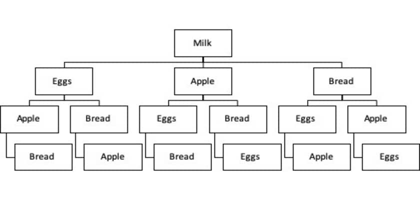
In this example, the algorithm first looks at level 1 which is Milk and finds it’s frequency, then it moves to the next depth layer and looks at frequencies of [Milk, Eggs], [Milk, Apple], and [Milk, Bread].
After second level of depth is analyzed, it moves on to the next depth level. This continues until it reaches the last depth level, which means that once there is no more new itemsets the algorithm will stop its calculation.
As an illustration, consider the above diagram, but now instead of items we will label the steps the algorithm takes:
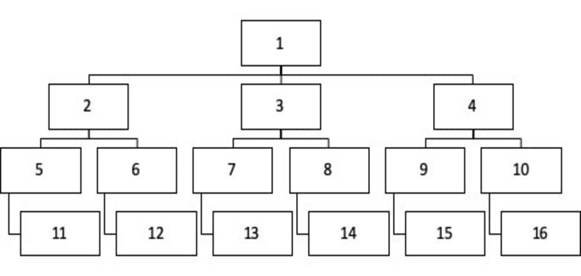
The diagram above shows the steps the algorithm takes while performing its search (1:16).
As a result, it calculates support for all possible combinations of itemsets.
Remember that it is up to us to set the minimum parameter values for support. If we set it to 0.01, we will obviously see much more possible rules than if we were to set it to 0.4.
The resulting output will be a list of association rules that were discovered while satisfying the parameter values that we set.
ECLAT (Explained with Examples)
The ECLAT algorithm is another popular tool for Market Basket Analysis. It stands for Equivalence Class Clustering and Bottom-Up Lattice Traversal. It is known as a “more efficient” Apriori algorithm.
It is a depth-first search (DFS) approach which searches vertically through a dataset structure. The algorithm starts its search at a tree root, then explores next depth level node and keeps going down until it reaches the first terminal node. Then it makes a step back (to n-1) level and explores other nodes and goes down to the terminal node.
It makes more sense when we explore it as a tree.
Recall the dataset we used in the Apriori Algorithm part. Here is how DFS would analyze it:
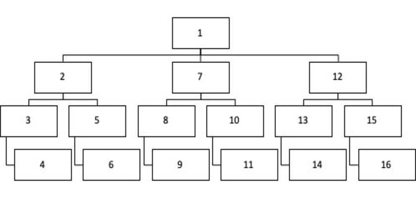
The steps ECLAT performs:
- Find the root (box 1).
- Explore next depth level nodes until you reach a terminal node (boxes 2:4).
- Once terminal node is reached (box 4), make a step back to a previous depth level and see if other nodes are available to explore (nothing at box 3 level).
- Make another step back (to box 2 level), now there is another “path” available (box 5).
- Go down until you reach terminal node (box 6).
- Keep repeating the above steps until there are no more nodes to explore.
If we compare it to Breadth-First Search (BFS), the computational speed will depend on the width and depth of the tree (different properties of the vertex orderings).
When it comes back to the technical part of ECLAT algorithm, its flow is the following:
- In the first run, ECLAT finds transaction IDs for all single-item itemsets (k=1).
- In the second run, ECLAT finds transaction IDs for all two-item itemsets (k=2).
- In the \(n^{th}\) run, ECLAT finds transaction IDs for all \(n\) -item itemsets (k=\(n\)).
Let’s put it to an example again. Here is our dataset:
$$
\begin{matrix}
\text{Transaction ID} & Milk & Eggs & Apples & Bread \\
001 & 1 & 1 & 0 & 1 \\
002 & 1 & 1 & 0 & 0 \\
003 & 1 & 0 & 0 & 1 \\
004 & 0 & 1 & 1 & 0 \\
\end{matrix}
$$
Below is a showcase of all the runs ECLAT algorithm will perform on this dataset:
- For k=1:
$$
\begin{matrix}
\begin{array}{c|c}
\text{Item} & \text{Transactions} \\
\hline
\text{Milk} & \text{001, 002, 003} \\
\text{Eggs} & \text{001, 002, 004} \\
\text{Apples} & \text{004} \\
\text{Bread} & \text{001, 003} \\
\end{array}
\end{matrix}
$$
- For k=2:
$$
\begin{matrix}
\begin{array}{c|c}
\text{Item} & \text{Transactions} \\
\hline
\text{Milk, Eggs} & \text{001, 002} \\
\text{Milk, Bread} & \text{001, 003} \\
\text{Eggs, Apples} & \text{004} \\
\text{Eggs, Bread} & \text{001} \\
\end{array}
\end{matrix}
$$
- For k=3:
$$
\begin{matrix}
\begin{array}{c|c}
\text{Item} & \text{Transactions} \\
\hline
\text{Milk, Eggs, Bread} & \text{001} \\
\end{array}
\end{matrix}
$$
- For k=4:
Once we reach four-item itemsets, we can see from our data that there aren’t any of them. In this case, the ECLAT algorithm will stop its search at k=3.
A few things to note:
- If two items don’t appear together on any transactions (such as {Milk, Apples}), it won’t appear in the matrix
- The matrix doesn’t contain duplicates ({Milk, Eggs} is the same as {Eggs, Milk}
Results:
Now, let’s say we have preset a minimum support count requirement equal to 2 (support count=2) for the ECLAT search.
This implies that for a rule to qualify for the output, it must have a minimum of 2 transactions where those items appear:
$$
\begin{matrix}
\begin{array}{c}
\text{Rule} \\
\hline
\text{Milk} \to \text{Eggs} \\
\text{Milk} \to \text{Bread} \\
\end{array}
\end{matrix}
$$
Note: support count and support are two different concepts. Support count (\(\sigma\)) is the count of transactions in which the item occurred. Support is the fraction of transactions where the item occurred of total number of transactions (support count divided by total number of transactions).
F-P Growth (Explained with Examples)
F-P Growth (or frequent-pattern growth) algorithm is another popular technique in Market Basket Analysis (first introduced by Han). It produces the same results as Apriori algorithm but is computationally faster due to a mathematically different technique (divide and conquer).
F-P Growth follows a two-step data preprocessing approach:
- First, it counts the number of occurrences of each item in the transactional dataset.
- Then, it creates a search-tree structure using the transactions.
Unlike Apriori algorithm, F-P Growth sorts items within each transaction by it’s frequency from largest to smallest before inserting it into a tree. This is where it has a substantial computational advantage over Apriori algorithm since it does the frequency sorting early on. Items which don’t meet minimum support (frequency) requirements (that we can set) are discarded from the tree.
Another advantage is that frequent itemsets that repeat will have the same path (unlike Apriori algorithm, where each itemset has a unique path).
Here is an example:
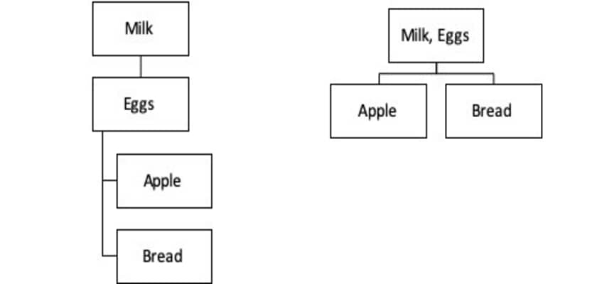
Left hand side is Apriori algorithm, and it looks at two individual sequences with these steps:
- Milk \(\to\) Eggs \(\to\) Apple
- Milk \(\to\) Eggs \(\to\) Bread
Right hand side is F-P Growth algorithm, and it looks at two sequences where the common part [Milk, Eggs] is compressed:
- [Milk, Eggs] \(\to\) Apple
- [Milk, Eggs] \(\to\) Bread
What this allows is a much higher compression towards the root of the tree and less computational steps (in this case 2 steps), which means that the calculation is much faster than Apriori algorithm (in this case 4 steps).
Comparison of Algorithms
This section is designed to give you a brief overview in a compare and contrast manner for the three algorithms studied in this course.
Please refer to the below table:
$$
\begin{matrix}
\begin{array}{|c|c|c|c|}
\text{Algorithm} & \text{Apriori} & \text{ECLAT} & \text{F-P Growth} \\
\hline
\text{Approach} & \text{BFS} & \text{DFS} & \text{Divide and conquer} \\
\text{Scan} & \text{Horizontal} & \text{Vertical} & \text{Horizontal} \\
\text{Structure} & \text{Array} & \text{Array} & \text{Tree} \\
\end{array}
\end{matrix}
$$
The above table suggests that the main speed advantages are due to a different computational technique and data format. Because F-P Growth goes through a database only twice, it is much faster on a large number of itemsets. In the example that we used, where the entire database consists of only 4 unique items, the computational speed difference will be minimal and not noticeable.
Association Rule Mining in Python (Example)
In this section we will create some examples of association rule mining in Python.
Let’s recall the dataset we created in one of the first parts of this article:
$$
\begin{matrix}
\text{Transaction ID} & Milk & Eggs & Apples & Bread \\
\hline
001 & 1 & 1 & 0 & 1 \\
002 & 1 & 1 & 0 & 0 \\
003 & 1 & 0 & 0 & 1 \\
004 & 0 & 1 & 1 & 0 \\
\end{matrix}
$$
We will use it as an input into our models.
To continue following this tutorial and perform association rule mining in Python we will need two Python libraries: pandas and mlxtend.
If you don’t have them installed, please open “Command Prompt” (on Windows) and install them using the following code:
pip install pandas
pip install mlxtend
Once the libraries are downloaded and installed, we can proceed with Python code implementation.
Step 1: Creating a list with the required data
dataset = [
    ["Milk", "Eggs", "Bread"],
    ["Milk", "Eggs"],
    ["Milk", "Bread"],
    ["Eggs", "Apple"],
]
The above code creates a list with transactions that we will use.
Let’s take a look at the result:
print(dataset)
[['Milk', 'Eggs', 'Bread'], ['Milk', 'Eggs'], ['Milk', 'Bread'], ['Eggs', 'Apple']]
Step 2: Convert list to dataframe with boolean values
import pandas as pd
from mlxtend.preprocessing import TransactionEncoder

te = TransactionEncoder()
te_array = te.fit(dataset).transform(dataset)
df = pd.DataFrame(te_array, columns=te.columns_)
We first import the required libraries. Then we save the TransactionEncoder() function as a local variable te.
Next step is to create an array (te_array) from the dataset list with True/False values (depending if an item appears/doesn’t appear on a particular receipt).
We then convert this array to a dataframe (df) using items as column names.
Let’s take a look at the result:
print(df)
   Apple  Bread   Eggs   Milk
0  False   True   True   True
1  False  False   True   True
2  False   True  False   True
3   True  False   True  False
This shows us across all of the transactions which items do/don’t occur on a particular receipt.
Step 3.1: Find frequently occurring itemsets using Apriori Algorithm
from mlxtend.frequent_patterns import apriori

frequent_itemsets_ap = apriori(df, min_support=0.01, use_colnames=True)
First, we import the apriori algorithm function from the library.
Then we apply the algorithm to our data to extract the itemsets that have a minimum support value of 0.01 (this parameter can be changed).
Let’s take a look at the result:
print(frequent_itemsets_ap)
   support             itemsets
0     0.25              (Apple)
1     0.50              (Bread)
2     0.75               (Eggs)
3     0.75               (Milk)
4     0.25        (Eggs, Apple)
5     0.25        (Eggs, Bread)
6     0.50        (Bread, Milk)
7     0.50         (Eggs, Milk)
8     0.25  (Eggs, Bread, Milk)
Step 3.2: Find frequently occurring itemsets using F-P Growth
from mlxtend.frequent_patterns import fpgrowth

frequent_itemsets_fp=fpgrowth(df, min_support=0.01, use_colnames=True)
First, we import the F-P growth algorithm function from the library.
Then we apply the algorithm to our data to extract the itemsets that have a minimum support value of 0.01 (this parameter can be tuned on a case-by-case basis).
Let’s take a look at the result:
print(frequent_itemsets_fp)
   support             itemsets
0     0.75               (Milk)
1     0.75               (Eggs)
2     0.50              (Bread)
3     0.25              (Apple)
4     0.50         (Eggs, Milk)
5     0.50        (Bread, Milk)
6     0.25        (Eggs, Bread)
7     0.25  (Eggs, Bread, Milk)
8     0.25        (Eggs, Apple)
Note: what you observe is regardless of the technique you used, you arrived at the identical itemsets and support values. The only difference is the order in which they appear. You should notice that the output from F-P Growth appears in descending orders, hence the proof of what we mentioned in the theoretical part about this algorithm.
Step 4: Mine the Association Rules
In this final step we will perform the association rule mining in Python for the frequent itemsets which we calculated in Step 3.
from mlxtend.frequent_patterns import association_rules

rules_ap = association_rules(frequent_itemsets_ap, metric="confidence", min_threshold=0.8)
rules_fp = association_rules(frequent_itemsets_fp, metric="confidence", min_threshold=0.8)
First we import the required function from the page to determine the association rules for a given dataset using some set of parameters.
Then we apply it to the two frequent item datasets which we created in Step 3.
Note: “metric” and “min_threshold” parameters can be tuned on a case-by-case basis, depending on the business problem requirements.
Let’s take a look at both sets of rules:
print(rules_ap)
     antecedents consequents  antecedent support  consequent support  support  confidence      lift  leverage  conviction
0        (Apple)      (Eggs)                0.25                0.75     0.25         1.0  1.333333    0.0625         inf
1        (Bread)      (Milk)                0.50                0.75     0.50         1.0  1.333333    0.1250         inf
2  (Eggs, Bread)      (Milk)                0.25                0.75     0.25         1.0  1.333333    0.0625         inf
print(rules_fp)
     antecedents consequents  antecedent support  consequent support  support  confidence      lift  leverage  conviction
0        (Bread)      (Milk)                0.50                0.75     0.50         1.0  1.333333    0.1250         inf
1  (Eggs, Bread)      (Milk)                0.25                0.75     0.25         1.0  1.333333    0.0625         inf
2        (Apple)      (Eggs)                0.25                0.75     0.25         1.0  1.333333    0.0625         inf
From the two above we see that both algorithms found identical association rules with same coefficients, just presented in a different order.
Conclusion
This article is a walkthrough for a basic example of implementation of association rule mining in Python for market basket analysis. We focused on theory and application of the most common algorithms.
There is much more to it:
- More algorithms
- More parameter tuning
- More data complexities
The purpose of this article is to showcase the possibilities of this data mining technique in application to market basket analysis in Python which can be definitely explored further.
Feel free to leave comments below if you have any questions or have suggestions for some edits and check out more of my Statistics articles.
References:
- Agrawal, R.; Imieliński, T.; Swami, A. (1993). “Mining association rules between sets of items in large databases”. Proceedings of the 1993 ACM SIGMOD international conference on Management of data – SIGMOD ’93. p. 207. CiteSeerX10.1.1.40.6984. doi:10.1145/170035.170072. ISBN978-0897915922.
- Han (2000). Mining Frequent Patterns Without Candidate Generation. Proceedings of the 2000 ACM SIGMOD International Conference on Management of Data. SIGMOD ’00. pp. 1–12. CiteSeerX10.1.1.40.4436. doi:10.1145/342009.335372.