In this article we will discuss the steps and intuition for matrix multiplication with examples using Python.
Table of contents
- Introduction
- What does a matrix represent
- Matrix vector multiplication explained
- Matrix vector multiplication explained graphically
- Matrix vector multiplication in Python
- Matrix multiplication explained
- Matrix multiplication explained graphically
- Matrix multiplication in Python
- Conclusion
Introduction
Matrix multiplication is one of the most popular topic in linear algebra, but often taught without explaining any intuition behind it. We all know the formulas, and use them all the time, but do we really understand the mechanics behind them?
When working with matrices, we use multiplication almost everywhere. A simple example would be checking if a calculated inverse of a matrix actually forms an identity matrix when multiplied by the original matrix.
In this article we explain the intuition and show graphical explanations of matrix by vector and matrix by matrix multiplication.
The examples used are fairly simple and don’t require even a calculator. However, the approaches learnt in this article can be applied on more complex matrix multiplications.
We also explore how quick and easy it is to perform matrix multiplication using Python.
To continue following this tutorial we will need the following Python library: numpy.
If you don’t have them installed, please open “Command Prompt” (on Windows) and install them using the following code:
pip install numpy
What does a matrix represent
To get started, we want to understand what a matrix really is and what does a matrix represent.
As an example, we will consider a 2×2 square matrix (where number of rows equals the number of columns), and let’s call it matrix \(A\):
$$A = \begin{bmatrix} 1 & 6 \\ 2 & 3\end{bmatrix}$$
The easiest way to think about a matrix in in terms of inputs and outputs, where the columns of a matrix represent the inputs and the rows represent the outputs:

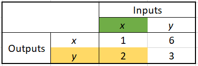
For example, for every \(X\) input (green) we will get:
an \(X\) output of \(1\) (yellow):

and a \(Y\) output of \(2\) (yellow):
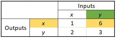
Similarly, for every \(Y\) input (green) we will get:
an \(X\) output of \(6\) (yellow):
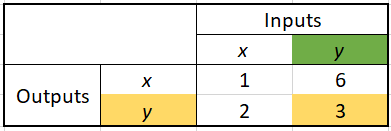
a \(Y\) output of \(3\) (yellow):
So far this should be a simple intuition. But the question is why do we even need it? And how can this be used?
An illustrative example follows in the next section, where we take this matrix \(A\) and try multiplying it by different vectors.
Matrix vector multiplication explained
In this section we will continue working with matrix \(A\):
$$A = \begin{bmatrix} 1 & 6 \\ 2 & 3 \end{bmatrix}$$
and explore how we can multiply it by different vectors and the intuition for this operation as well as the output.
Example 1 – Multiply matrix by \(\begin{bmatrix} 1 \\ 0 \end{bmatrix} \)vector:
Let’s say we would like to multiply matrix \(A\) by vector \(b = \begin{bmatrix} 1 \\ 0 \end{bmatrix} \):
$$ A \times b = \begin{bmatrix} 1 & 6 \\ 2 & 3 \end{bmatrix} \times \begin{bmatrix} 1 \\ 0 \end{bmatrix} = ?$$
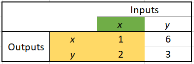
We see that vector \(\begin{bmatrix} 1 \\ 0 \end{bmatrix} \) is only \(X\) input, so we can go back to the table and ask: what are the \(X\) and \(Y\) for every \(X\) input?
We can see that for \(1\) \(X\) input, the output is \(1\) \(X\) and \(2\) \(Y\):
such that:
$$A \times b = \begin{bmatrix} 1 & 6 \\ 2 & 3 \end{bmatrix} \times \begin{bmatrix} 1 \\ 0 \end{bmatrix} = \begin{bmatrix} 1 \\ 2 \end{bmatrix}$$
Example 2 – Multiply matrix by \(\begin{bmatrix} 0 \\ 1 \end{bmatrix} \)vector:
In this example. let’s say we would like to multiply matrix \(A\) by vector \(c = \begin{bmatrix} 0 \\ 1 \end{bmatrix} \):
$$A \times c = \begin{bmatrix} 1 & 6 \\ 2 & 3 \end{bmatrix} \times \begin{bmatrix} 0 \\ 1 \end{bmatrix} = ?$$
We see that vector \(\begin{bmatrix} 0 \\ 1 \end{bmatrix} \) is only \(Y\) input, so we can go back to the table and ask: what are the \(X\) and \(Y\) for every \(Y\) input?
We can see that for \(1\) \( Y\) input, the output is \(6\) \(X\) and \(3\) \(Y\):

such that:
$$A \times c = \begin{bmatrix} 1 & 6 \\ 2 & 3 \end{bmatrix} \times \begin{bmatrix} 0 \\ 1 \end{bmatrix} = \begin{bmatrix} 6 \\ 3 \end{bmatrix}$$
Example 3 – Multiply matrix by \(\begin{bmatrix} 3 \\ 2 \end{bmatrix} \) vector:
In this example, we combine the logic from the previous two examples and look at the multiplication of a matrix by vector \(d = \begin{bmatrix} 3 \\ 2 \end{bmatrix} \) with both \(X\) and \(Y\) values:
$$A \times d = \begin{bmatrix} 1 & 6 \\ 2 & 3 \end{bmatrix} \times \begin{bmatrix} 3 \\ 2 \end{bmatrix} = ?$$
We already know the outputs for every \(1\) \(X\) and \(1\) \(Y\) inputs. But how does it change for larger numbers?
The output is simply multiplied by the input value. Let’s see how we calculate it!
For \(X\) input, we now have an input of \(3\) \(X\). Knowing that the output for each \(1\) \(X\) value is \(\begin{bmatrix} 1 \\ 2 \end{bmatrix}\), then for \(3\) \(X\) values it’s: \(\begin{bmatrix} 1 \times 3 \\ 2 \times 3 \end{bmatrix} = \begin{bmatrix} 3 \\ 6 \end{bmatrix} \)
For \(Y\) input, we now have an input of \(2\) \(Y\). Knowing that the output for each \(1\) \(Y\) value is \(\begin{bmatrix} 6 \\ 3 \end{bmatrix}\), then for \(2\) \(Y\) values it’s: \(\begin{bmatrix} 6 \times 2 \\ 3 \times 2 \end{bmatrix} = \begin{bmatrix} 12 \\ 6 \end{bmatrix} \)
And finally, we will need to add these two intermediate results together:
$$\begin{bmatrix} 3 \\ 6 \end{bmatrix} + \begin{bmatrix} 12 \\ 6 \end{bmatrix} = \begin{bmatrix} 3+12 \\ 6+6 \end{bmatrix} = \begin{bmatrix} 15 \\ 12 \end{bmatrix} $$
therefore:
$$A \times d = \begin{bmatrix} 1 & 6 \\ 2 & 3 \end{bmatrix} \times \begin{bmatrix} 3 \\ 2 \end{bmatrix} = \begin{bmatrix} 15 \\ 12 \end{bmatrix} $$
Using these steps you can perform matrix multiplication using any values.
Matrix vector multiplication explained graphically
We continue to work with matrix \(A\):
$$A = \begin{bmatrix} 1 & 6 \\ 2 & 3\end{bmatrix}$$
and now think of it as two separate vectors which together create this matrix.
The original base vectors are \(\vec{v}_1 = (1, 0)\) and \(\vec{v}_2 = (0, 1)\), but after applying matrix \(A\) on them, we see how they shift and become:
$$\vec{v}_1 = (1, 2)$$
$$\vec{v}_2 = (6, 3)$$
and they are the shifted base vectors:
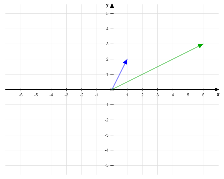
And vector \(d = \begin{bmatrix} 3 \\ 2 \end{bmatrix} \) (by which we multiply) represents the scalars for the base vectors \(\vec{v}_1\) and \(\vec{v}_2\).
What does this mean when it comes down to multiplication in our example? It means that we will first multiply each base vector (\(\vec{v}_1\) and \(\vec{v}_2\)) by their scalars (3 and 2 respectively), and then find the sum of the resulting vectors.
The new vectors are:
$$\vec{v}_1^n = 3 \times \vec{v}_1 = 3\times(1, 2) = (3\times 1, 3 \times 2) = (3, 6) $$
$$\vec{v}_2^n = 2 \times \vec{v}_2 = 2\times(6, 3) = (2\times 6, 2 \times 3) = (12, 6) $$
and graphically:
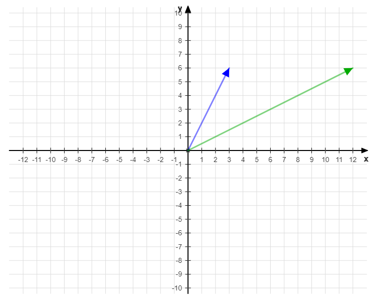
where \(\vec{v}_1\) moved to \(\vec{v}_1^n\) (blue vector), and \(\vec{v}_2\) moved to \(\vec{v}_2^n\) (green vector).
Now, the final step is to find the sum of \(\vec{v}_1^n\) and \(\vec{v}_2^n\) (\(\vec{v}_1^n + \vec{v}_2^n\)), which is the red vector shown below:
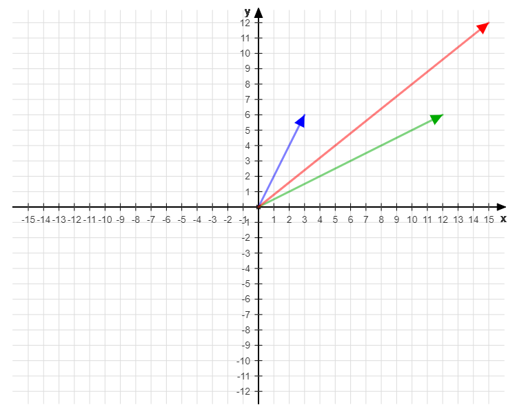
The coordinates of the resulting vector are (15, 12), which is exactly the same resulting vector as in the linear algebra solution, such that:
$$A \times d = \begin{bmatrix} 1 & 6 \\ 2 & 3 \end{bmatrix} \times \begin{bmatrix} 3 \\ 2 \end{bmatrix} = \begin{bmatrix} 15 \\ 12 \end{bmatrix} $$
Matrix vector multiplication in Python
In order to perform the matrix vector multiplication in Python we will use the numpy library. And the first step will be to import it:
import numpy as np
Numpy has a lot of useful functions, and for this operation we will use the matmul() function which computes the matrix product of two arrays.
Recall that in Python matrices are constructed as arrays. And the next step will be to define the input matrices. We are going to use the same 2×2 and 2×1 matrices as in Example 3 from the previous section:
A = np.array([[1, 6],
              [2, 3]])

d = np.array([[3],
              [2]])
Now that we have the required matrices, we can easily calculate the matrix resulting from multiplication:
result = np.matmul(A,d)

print(result)
And you should get:
[[15]
 [12]]
which is exactly the same output as in our example where we calculated it manually.
Matrix multiplication explained
This section is simply an extension of the matrix vector multiplication explanation.
We will continue working with matrix \(A\):
$$A = \begin{bmatrix} 1 & 6 \\ 2 & 3 \end{bmatrix}$$
And now we will try to multiply it by another matrix, \(B\):
$$B = \begin{bmatrix} 5 & 1 \\ 3 & 2 \end{bmatrix}$$
So that we have:
$$A \times B = \begin{bmatrix} 1 & 6 \\ 2 & 3 \end{bmatrix} \times \begin{bmatrix} 5 & 1 \\ 3 & 2 \end{bmatrix} = ?$$
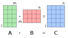
One important thing to note about matrix multiplication is that the number of rows if the first matrix (matrix \(A\)) must be equal to the number of columns in the second matrix (matrix \(B\)). And the resulting matrix (\(A \times B\)) should have the number of rows of the first matrix (matrix \(A\)) ane the number of columns of the second matrix (matrix \(B\)), such that:
How can we simplify the calculation of \(A \times B\)?
What we will do is try to separate matrix \(B\) into two vectors in our imagination by drawing an imaginary line between two columns:

Then we can perform the matrix vector multiplication on each vector, and glue the resulting vectors together in one matrix.
As you can imagine there will be three steps here:
Step 1:
Calculate the left part of the resulting matrix:
$$A \times \begin{bmatrix} 5 \\ 3 \end{bmatrix} = \begin{bmatrix} 1 & 6 \\ 2 & 3 \end{bmatrix} \times \begin{bmatrix} 5 \\ 3 \end{bmatrix} = \begin{bmatrix} 23 \\ 19 \end{bmatrix}$$
Step 2:
Calculate the right part of the resulting matrix:
$$A \times \begin{bmatrix} 1 \\ 2 \end{bmatrix} = \begin{bmatrix} 1 & 6 \\ 2 & 3 \end{bmatrix} \times \begin{bmatrix} 1 \\ 2 \end{bmatrix} = \begin{bmatrix} 13 \\ 8 \end{bmatrix}$$
Step 3:
Write the resulting matrix as:
$$A \times B = \begin{bmatrix} 1 & 6 \\ 2 & 3 \end{bmatrix} \times \begin{bmatrix} 5 & 1 \\ 3 & 2 \end{bmatrix} = \begin{bmatrix} 23 & 13 \\ 19 & 8 \end{bmatrix}$$
Matrix multiplication explained graphically
We will use the same matrices as in the explanation section:
$$A = \begin{bmatrix} 1 & 6 \\ 2 & 3 \end{bmatrix}$$
$$B = \begin{bmatrix} 5 & 1 \\ 3 & 2 \end{bmatrix}$$
And let’s again imagine that we can split matrix \(B\) into two vectors like this:

We take matrix \(A\) and think of it as two separate vectors than together create this matrix.
The original base vectors are \(\vec{v}_1 = (1, 0)\) and \(\vec{v}_2 = (0, 1)\), but after applying matrix \(A\) on them, we see how they shift and become:
$$\vec{v}_1 = (1, 2)$$
$$\vec{v}_2 = (6, 3)$$
and they are the shifted base vectors:

And matrix \(B\) (by which we multiply) represents the two vectors scalars for the base vectors \(\vec{v}_1\) and \(\vec{v}_2\).
What does this mean when it comes down to multiplication in our example?
Step 1:
First we will multiply each base vector (\(\vec{v}_1\) and \(\vec{v}_2\)) by their scalars (5 and 3 respectively) from the left half of matrix \(B\), and then find the sum of the resulting vectors.
This will give us:
$$\vec{v}_1^{nl} = 5 \times \vec{v}_1 = 5\times(1, 2) = (5\times 1, 5 \times 2) = (5, 10) $$
$$\vec{v}_2^{nl} = 3 \times \vec{v}_2 = 3\times(6, 3) = (3\times 6, 3 \times 3) = (18, 9) $$
and graphically:
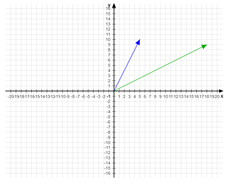
where \(\vec{v}_1\) moved to \(\vec{v}_1^{nl}\) (blue vector), and \(\vec{v}_2\) moved to \(\vec{v}_2^{nl}\) (green vector).
Now, the final step is to find the sum of \(\vec{v}_1^{nl}\) and \(\vec{v}_2^{nl}\) (\(\vec{v}_1^{nl} + \vec{v}_2^{nl}\)), which is the red vector shown below:
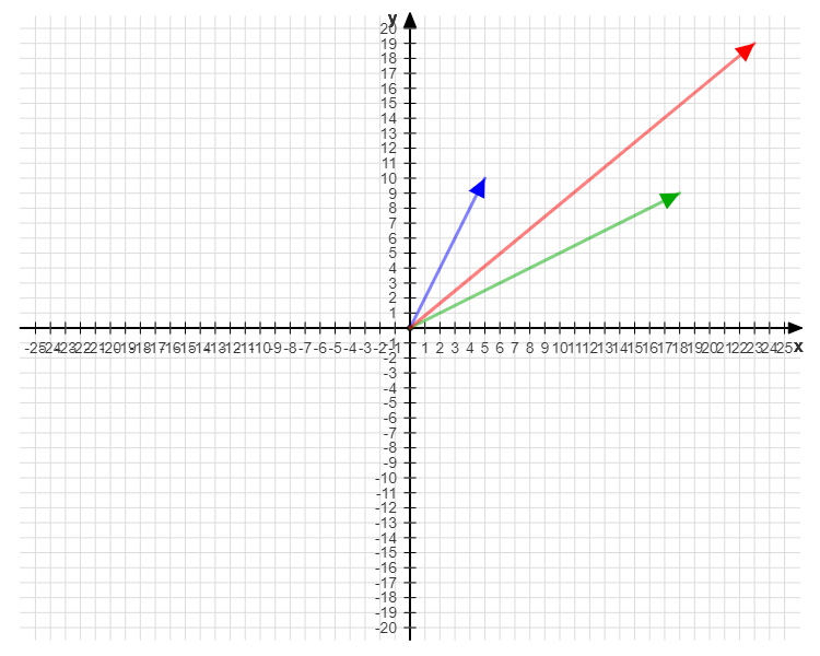
and this now solves the left half of our result matrix with this summation vector being (29, 19).
Step 2:
Then, we will multiply each base vector (\(\vec{v}_1\) and \(\vec{v}_2\)) by their scalars (1 and 2 respectively) from the right half of matrix \(B\), and then find the sum of the resulting vectors.
This will give us:
$$\vec{v}_1^{nr} = 1 \times \vec{v}_1 = 1\times(1, 2) = (1\times 1, 1 \times 2) = (1, 2) $$
$$\vec{v}_2^{nr} = 2 \times \vec{v}_2 = 2\times(6, 3) = (2\times 6, 2 \times 3) = (12, 6) $$
and graphically:
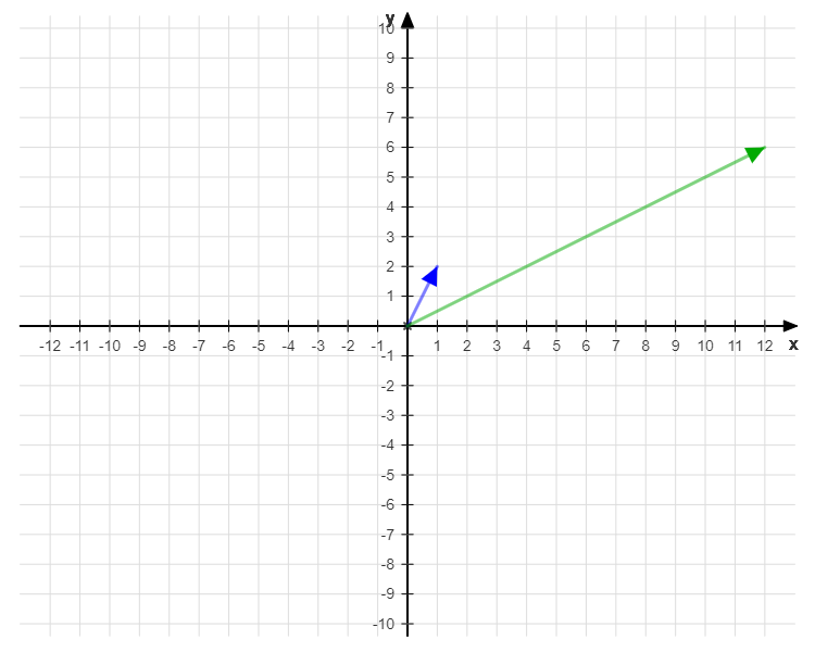
where \(\vec{v}_1\) moved to \(\vec{v}_1^{nr}\) (blue vector), and \(\vec{v}_2\) moved to \(\vec{v}_2^{nr}\) (green vector).
Now, the final step is to find the sum of \(\vec{v}_1^{nr}\) and \(\vec{v}_2^{nr}\) (\(\vec{v}_1^{nr} + \vec{v}_2^{nr}\)), which is the red vector shown below:
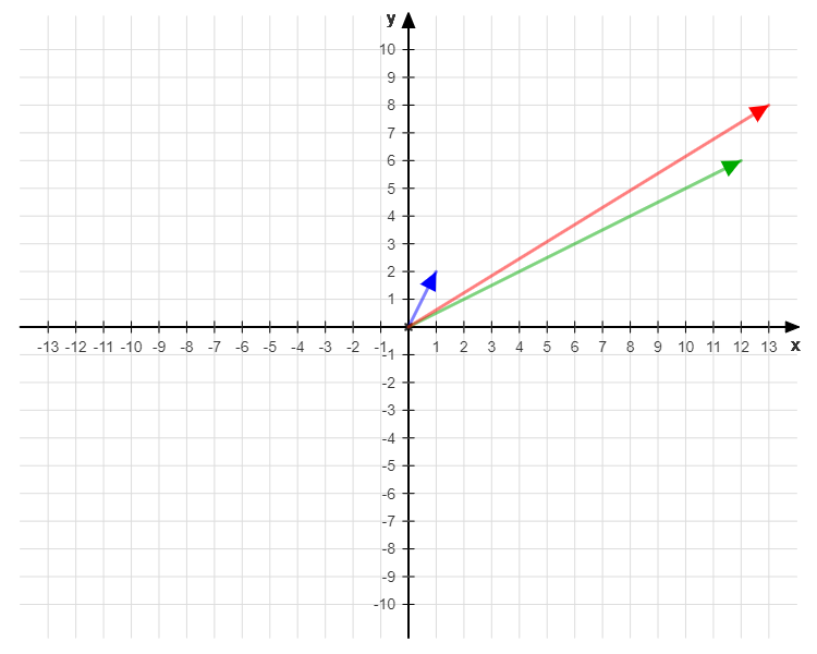
and this now solves the left half of our result matrix with this summation vector being (13, 8).
Step 3:
Combine the results from previous steps, or basically “glue” two resulting vectors into one matrix.
From Step 1 we have the resulting vector (29, 19), and from Step 2 we have the resulting vector (13, 8).
Putting it together in a matrix:
$$\begin{bmatrix} 23 & 13 \\ 19 & 8 \end{bmatrix}$$
which is exactly the same resulting matrix as in the linear algebra solution, such that:
$$A \times B = \begin{bmatrix} 1 & 6 \\ 2 & 3 \end{bmatrix} \times \begin{bmatrix} 5 & 1 \\ 3 & 2 \end{bmatrix} = \begin{bmatrix} 23 & 13 \\ 19 & 8 \end{bmatrix}$$
Matrix multiplication in Python
In order to perform the matrix vector multiplication in Python we will use the numpy library. And the first step will be to import it:
import numpy as np
Numpy has a lot of useful functions, and for this operation we will use the matmul() function which computes the matrix product of two arrays.
Recall that in Python matrices are constructed as arrays. And the next step will be to define the input matrices. We are going to use the same 2×2 and 2×2 matrices as in example from the previous section:
A = np.array([[1, 6],
              [2, 3]])

B = np.array([[5, 1],
              [3, 2]])
Now that we have the required matrices, we can easily calculate the matrix resulting from multiplication:
result = np.matmul(A, B)

print(result)
And you should get:
[[23 13]
 [19  8]]
which is exactly the same output as in our example where we calculated it manually.
Conclusion
In this article we discussed the intuition behind matrix by vector and matrix by matrix multiplication using both linear algebra and graphic approaches, as well as shown complete examples using Python.
Feel free to leave comments below if you have any questions or have suggestions for some edits and check out more of my Linear Algebra articles.

In python 3.5 and higher, you can use for matrix multiply, operator @ (built-in operator for matrices multiplication)