In this tutorial we will explore how to calculate skewness in Python.
Table of contents
- Introduction
- What is skewness?
- How to calculate skewness?
- How to calculate skewness in Python?
- Conclusion
Introduction
Skewness is something we observe in many areas of our daily lives. For example, something that people often search online is salary distribution in a particular country of interest. Here is an example:

Find more statistics at Statista
Looking at Canadian distribution of income in 2019, we can see that the average income is somewhere between $40,000-$50,000 approximately from the above graph.
What we also notice is that the data is not normally distributed around the mean, therefore having some type of skew.
In the above example, there is clearly some negative skew with a thicker left tail of the distribution. But why is there a skew? We see that the median of the distribution will be around $60,000, so it is larger than the mean; and the mode of the distribution will be between $60,000 and $70,000, thus creating the skew we observe above.
Where kurtosis measures whether there are extreme values in either of the tails (or simply if the tails are heavy or light), skewness focuses on the differentiating the tails of the distribution based on the extreme values (or simply the symmetry of the tails)
To continue following this tutorial we will need the following Python library: scipy.
If you don’t have it installed, please open “Command Prompt” (on Windows) and install it using the following code:
pip install scipy
What is skewness?
In statistics, skewness is a measure of asymmetry of the probability distribution about its mean and helps describe the shape of the probability distribution. Basically it measures the level of how much a given distribution is different from a normal distribution (which is symmetric).
Skewness can take several values:
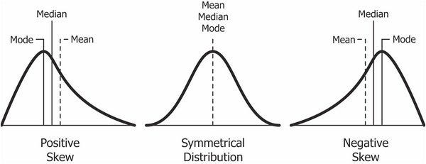
- Positive – observed when the distribution has a thicker right tail and mode<median<mean.
- Negative – observed when the distribution has a thicker left tail and mode>median>mean.
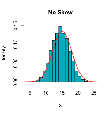
- Zero (or nearly zero) – observed when the distribution is symmetric about its mean and approximately mode=median=mean.
Note: the above definitions are generalized and values can differ in signs based on families of distributions.
How to calculate skewness?
In most cases, the sample skewness is calculated as the Fisher-Pearson coefficient of skewness (Note: there are more ways of calculating skewness: Bowley, Kelly’s measure, Momental).
This method looks at the measure of skewness as the third standardized moment of a distribution.
Sounds a bit complicated? Follow the next steps to have a complete understanding of the calculations.
The \(k^{th}\) moment of the distribution can be calculated as:
$$\widetilde{\mu}_{k} = \frac{\mu_{k}}{\sigma_{k}} = \frac{E[(X-\mu)^k]}{(E[(X-\mu)^2])^{\frac{k}{2}}}$$
As mentioned before, skewness is the third moment of the distribution and can be calculated as:
$$g_1 = \frac{m_3}{(m_2)^\frac{3}{2}}$$
where:
$$m_k = \frac{1}{N} \sum_{n=1}^{N}(x_n – \bar{x})^k$$
If you want to correct for statistical bias, then you should solve for the adjusted Fisher-Pearson standardized moment coefficient as:
$$G_1 = \frac{k_3}{(k_2)^\frac{3}{2}} = \frac{\sqrt{N(N-1)}}{N-2} \times \frac{m_3}{(m_2)^\frac{3}{2}}$$
Example:
It is a lot of formulas above. To make it all into a better understandable concept let’s take a look at an example!
Consider the following sequence of 10 numbers that represent students’ grades on a test:
\(X\) = [55, 78, 65, 98, 97, 60, 67, 65, 83, 65]Calculating the mean of X we get: \(\bar{x}=73.3\).
Solving for \(m_3\):
$$m_3 = \frac{1}{10}\sum_{n=1}^{10}(x_n – \bar{x})^3$$
$$m_3 = \frac{(55-73.3)^3 – (78-73.3)^3 – … – (65-73.3)^3}{10} = 1,895.124$$
Solving for \(m_2\):
$$m_2 = \frac{1}{10}\sum_{n=1}^{10}(x_n – \bar{x})^2$$
$$m_2 = \frac{(55-73.3)^2 – (78-73.3)^2 – … – (65-73.3)^2}{10} = 204.61$$
Solving for \(g_1\):
$$g_1 = \frac{m_3}{(m_2)^\frac{3}{2}} = \frac{1,895.124}{(204.61)^\frac{3}{2}} = 0.647511$$
The Fisher-Pearson coefficient of skewness is equal to 0.647511 in this example and show that there is a positive skew in the data. Another way to check it is to look at the mode, median, and mean for these values. Here we have mode<mean<median with values 65<66<73.3.
In addition, let’s calculate the adjusted Fisher-Pearson coefficient of skewness:
$$G_1 = \frac{\sqrt{N(N-1)}}{N-2} \times \frac{m_3}{(m_2)^\frac{3}{2}} = \frac {\sqrt{10(9)}}{8} \times \frac{1,895.124}{(204.61)^\frac{3}{2}} = 0.767854$$
How to calculate Skewness in Python?
In this section we will go through an example of calculating skewness in Python.
First, let’s create a list of numbers like the one in the previous part:
x =[55, 78, 65, 98, 97, 60, 67, 65, 83, 65]
To calculate the Fisher-Pearson correlation of skewness, we will need the scipy.stats.skew function:
from scipy.stats import skew
To calculate the unadjusted skewness in Python, simply run:
print(skew(x))
And we should get:
0.6475112950060684To calculate the adjusted skewness in Python, pass bias=False as an argument to the skew() function:
print(skew(x, bias=False))
And we should get:
0.7678539385891452Conclusion
In this article we discussed how to calculate skewness for a set of numbers in Python using scipy library.
Feel free to leave comments below if you have any questions or have suggestions for some edits and check out more of my Statistics articles.