In this tutorial we will explore how to test for normality using Python.
Table of contents
- Introduction
- Sample data for normality testing
- Q-Q plot in Python
- Jarque-Bera test in Python
- Kolmogorov-Smirnov test in Python
- Anderson-Darling test in Python
- Shapiro-Wilk test in Python
- Normality test results comparison
- Conclusion
Introduction
In this tutorial we will perform Jarque-Bera test in Python, Kolmogorov-Smirnov test in Python, Anderson-Darling test in Python, and Shapiro-Wilk test in Python on a sample data of 52 observations on returns of Microsoft stock.
We will also compare the results of each test and mention their advantages and disadvantages.
To continue following this tutorial we will need the following Python libraries: pandas, numpy, matplotlib, seaborn, and scipy.
If you don’t have it installed, please open “Command Prompt” (on Windows) and install it using the following code:
pip install pandas
pip install numpy
pip install matplotlib
pip install seaborn
pip install scipy
Sample data for normality testing
In this article we will be working with weekly historical returns on Microsoft stock. Let’s consider the period between 01/01/2018 and 31/12/2018. This data can be easily downloaded from Yahoo! finance.
Go ahead and download the data in .csv format and save it in the same directory as the .py file with the code we will build.
Now that we have the data downloaded, let’s import it in Python and select the columns that have the date of observation and the closing price:
import pandas as pd

df = pd.read_csv('MSFT.csv')
df = df[['Date', 'Close']]
Displaying first few rows of the data with stock prices:
print(df.head(3))
We should get:
         Date      Close
0  2018-01-01  88.190002
1  2018-01-08  89.599998
2  2018-01-15  90.000000
As you will see, the file contains data on Microsoft stock price for 53 weeks. Now, we want to work with returns on the stock, not the price itself, so we will need to do a little bit of data manipulation:
df['diff'] = pd.Series(np.diff(df['Close']))
df['return'] = df['diff']/df['Close']

df = df[['Date', 'return']].dropna()
Displaying first few rows of the data with stock returns:
print(df.head(3))
We should get:
         Date    return
0  2018-01-01  0.015988
1  2018-01-08  0.004464
2  2018-01-15  0.045111
To make more sense of this data, and particularly why we have converted prices to returns which we then want to test for normality using Python, let’s visualize the data using a histogram:
from matplotlib import pyplot as plt

plt.hist(df['return'])
plt.show()
And we get:
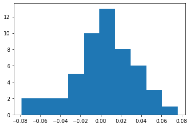
Notice that the distribution of data visually looks somewhat like normal distribution. But is it really? That is the question we are going to answer using different statistical methods in the following sections!
Q-Q plot in Python
We will start with one of the more visual and less mathematical approaches, quantile-quantile plot.
What is a quantile-quantile plot? It is a plot that shows the distribution of a given data against normal distribution, namely existing quantiles vs normal theoretical quantiles.
Let’s create the Q-Q plot for our data using Python and then interpret the results.
import pylab
import scipy.stats as stats

stats.probplot(df['return'], dist="norm", plot=pylab)
pylab.show()
And we should get:
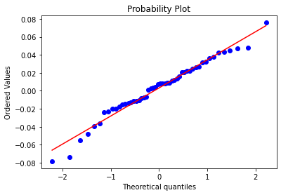
Looking at the graph above, we see an upward sloping linear relationship. For a normal distribution, the observations should all occur on the 45 degree straight line. Do we see such relationship above? We do partially. So what this can signal to us is that the distribution we are working with is not perfectly normal but close to it.
Jarque–Bera test in Python
Jarque-Bera is one of the normality tests or specifically a goodness of fit test of matching skewness and kurtosis to that of a normal distribution.
Its statistic is non-negative and large values signal significant deviation from normal distribution.
The test statistic JB of Jarque-Bera is defined by:
$$JB = \frac{n}{6} \times \bigg(S^2 + \frac{(K-3)^2}{4} \bigg)$$
where \(S\) is the sample skewness, \(K\) is the sample kurtosis, and \(n\) is the sample size.
The hypotheses:
$$H_0: \textit{sample } S \textit{ and sample } K \textit{ is not significantly different from normal distribution}$$
$$H_1: \textit{sample } S \textit{ and sample } K \textit{ is significantly different from normal distribution}$$
Now we can calculate the Jarque-Bera test statistic in Python and find the corresponding \(p\)-value:
from scipy.stats import jarque_bera

result = (jarque_bera(df['return']))

print(f"JB statistic: {result[0]}")
print(f"p-value: {result[1]}")
And we should get:
JB statistic: 1.937410519618088
p-value: 0.37957417002405025
Looking at these results, we fail to reject the null hypothesis and conclude that the sample data follows normal distribution.
Note: Jarque-Bera test works properly in large samples (usually larger than 2000 observations) at its statistic has a Chi-squared distribution with 2 degrees of freedom).
Kolmogorov-Smirnov test in Python
One of the most frequently tests for normality is the Kolmogorov-Smirnov test (or K-S test). A major advantage compared to other tests is that Kolmogorov-Smirnov test is nonparametric, meaning that it is distribution-free.
Here we focus on the one-sample Kolmogorov-Smirnov test because we are looking to compare a one-dimensional probability distribution with a theoretically specified distribution (in our case it is normal distribution).
The Kolmogorov-Smirnov test statistic measures the distance between the empirical distribution function (ECDF) of the sample and the cumulative distribution function of the reference distribution.
In our example, the empirical distribution function will come from the data on returns we have compiled earlier. And since we are comparing it to normal distribution, we will work with cumulative distribution function of the normal distribution.
So far this sounds very technical, so let’s try to break it down and visualize for better understanding.
Step 1:
Let’s create an array of values from a normal distribution with mean and standard deviation of our returns data:
import numpy as np

data_norm = np.random.normal(np.mean(df['return']), np.std(df['return']), len(df))
Using np.random.normal() we created the data_norm which is an array that has the same number of observations as df[‘return’] and also has the same mean and standard deviation.
The intuition here would be that we if we assume some parameters of the distribution (mean and standard deviation), what would be the numbers with such parameters that would form a normal distribution.
Step 2:
Next, what we are going to do is use np.histogram() on both datasets to sort them and allocate to bins:
values, base = np.histogram(df['return'])
values_norm, base_norm = np.histogram(data_norm)
Note: by default, the function will use bins=10, which you can adjust based on the data you are working with.
Step 3:
Use np.cumsum() to calculate cumulative sums of arrays created above:
cumulative = np.cumsum(values)
cumulative_norm = np.cumsum(values_norm)
Step 4:
Plot the cumulative distribution functions:
plt.plot(base[:-1], cumulative, c='blue')
plt.plot(base_norm[:-1], cumulative_norm, c='green')
plt.show()
And you should get:
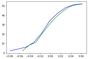
Where the blue line is the ECDF (empirical cumulative distribution function) of df[‘return’], and the green line is the CDF of a normal distribution.
Step 4 Alternative:
You can create the graph quicker by using seaborn and only need df[‘return’] and data_norm from Step 1:
import seaborn as sns

sns.ecdfplot(df['return'], c='blue')
sns.ecdfplot(data_norm, c='green')
And you should get:
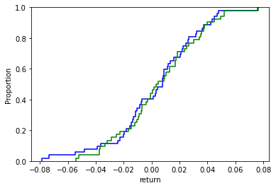
Let’s go back to the Kolmogorov-Smirnov test now after visualizing these two cumulative distribution functions. Kolmogorov-Smirnov test is based on the maximum distance between these two curves (blue – green) with the following hypotheses:
$$H_0: \textit{ two samples are from the same distribution}$$
$$H_1: \textit{ two samples are from different distributions} $$
We define ECDF as:
$$F_n(x) = P_n(X \leq x) = \frac{1}{n} \sum^{n}_{i=1}I(X_i \leq x)$$
which counts the proportion of the sample observations below level \(x\).
We define a given (theoretical) CDF as: \(F(x)\). In case of testing for normality, \(F(x)\) is the CDF of a normal distribution.
The Kolmogorov-Smirnov statistic is defined as:
$$D_n = \sup_{x}|F_n(x) – F(x)|$$
Intuitively, this statistic measures the largest absolute distance between two distribution functions for all \(x\) values.
Using the graph above, here is my estimated supremum:
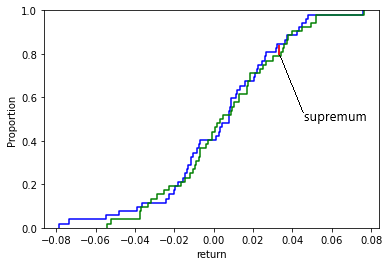
Calculating the value of \(D_n\) and comparing it with the critical value (assume 5%) of \(D_{0.05}\), we can either reject or fail to reject the null hypothesis.
Back to our example, let’s perform the K-S test in Python for the Microsoft stock returns data:
from scipy.stats import kstest

result = (kstest(df['return'], cdf='norm'))

print(f"K-S statistic: {result[0]}")
print(f"p-value: {result[1]}")
And we should get:
K-S statistic: 0.46976096086398267
p-value: 4.788934452701707e-11
Since the \(p\)-value is significantly less than 0.05, we reject the null hypothesis and accept the alternative hypothesis that two samples tested are not from the same cumulative distribution, meaning that the returns on Microsoft stock are not normally distributed.
Anderson-Darling test in Python
Anderson-Darling test (A-D test) is a modification of Kolmogorov-Smirnov test described above. It tests whether a given sample of observations is drawn from a given probability distribution (in our case from normal distribution).
$$H_0: \textit{ the data comes from a specified distribution}$$
$$H_1: \textit{ the data doesn’t come from a specified distribution} $$
A-D test is more powerful than K-S test since it considers all of the values in the data and not just the one that produces maximum distance (like in K-S test). It also assigns more weight to the tails of a fitted distribution.
This test belongs to the quadratic empirical distribution function (EDF) statistics, and is given by:
$$A^2 = n \int_{-\infty}^{\infty} \bigg (F_n(x) – F(x) \bigg )^2 w(x) dF(x)$$
where \(F\) is the hypothesized distribution (in our case, normal distribution), \(F_n\) is the ECDF (calculations discussed in the previous section), and \(w(x)\) is the weighting function.
The weighting function is given by:
$$w(x) = \bigg[F(x)(1-F(x))\bigg]^{-1}$$
which allows to place more weight on observations in the tails of the distribution.
Given such a weighting function, the test statistic can be simplified to:
$$A^2 = n \int_{-\infty}^{\infty} \frac{(F_n(x) – F(x))^2}{ F(x)(1-F(x))} dF(x)$$
Suppose we have a sample of data \(X\) and we want to test whether this sample comes from a cumulative distribution function (\(F(x)\)) of the normal distribution.
We need to sort the data such that \({x_1 < x_2 < … < x_n}\) and then compute the \(A^2\) statistic as:
$$A^2 = -n – \sum^{n}_{i=1} \frac{2i – 1}{n} \bigg [ln(F(x_i)) + ln(1 – F(x_{n+1-i})) \bigg ]$$
Back to our example, let’s perform the A-D test in Python for the Microsoft stock returns data:
from scipy.stats import anderson

result = (anderson(df['return'], dist='norm'))

print(f"A-D statistic: {result[0]}")
print(f"Critical values: {result[1]}")
print(f"Significance levels: {result[2]}")
And we should get:
A-D statistic: 0.3693823006816217
Critical values: [0.539 0.614 0.737 0.86  1.023]
Significance levels: [15.  10.   5.   2.5  1. ]
The first row of the output is the A-D test statistic, which is around 0.37; the third row of the output is a list with different significance levels (from 15% to 1%); the second row of the output is a list of critical values for the corresponding significance levels.
Let’s say we want to test our hypothesis at the 5% level, meaning that the critical value we will use is 0.737 (from the output above). Since the computer A-D test statistic (0.37) is less than the critical value (0.737), we fail to reject the null hypothesis and conclude that the sample data of Microsoft stock returns comes from a normal distribution.
Shapiro-Wilk test in Python
Shapiro-Wilk test (S-W test) is another test for normality in statistics with the following hypotheses:
$$H_0: \textit{ distribution of the sample is not significantly different from a normal distribution}$$
$$H_1: \textit{ distribution of the sample is significantly different from a normal distribution}$$
Unlike Kolmogorov-Smirnov test and Anderson-Darling test, it doesn’t base its statistic calculation on ECDF and CDF, rather it uses constants generated from moments from a normally distributed sample.
The Sharpiro-Wilk test statistics is defined as:
$$W = \frac{(\sum^n_{i=1} a_i x_{(i)})^2}{\sum^n_{i=1}(x_i – \bar{x})^2}$$
where \(x_{(i)}\) is the \(i\)th smallest number in the sample (\(x_{1}< x_{2}<…< x_{n} \)); and \(a_i\) are constants generated from var, cov, mean for a normally distributed sample.
Back to our example, let’s perform the S-W test in Python for the Microsoft stock returns data:
from scipy.stats import shapiro

result = (shapiro(df['return']))

print(f"S-W statistic: {result[0]}")
print(f"p-value: {result[1]}")
And we should get:
S-W statistic: 0.9772366881370544
p-value: 0.41611215472221375
Given the large \(p\)-value (0.42) which is greater than 0.05 (>0.05), we fail to reject the null hypothesis and conclude that the sample sample is not significantly different from a normal distribution.
Note: one of the biggest limitations of this test is the size bias, meaning that the larger the size of the sample is, the more likely you are to get a statistically significant result.
Normality test results comparison
Below is a table with results for the normality tests discussed in this article and their performance using a sample size of 52 observations on returns of Microsoft stock.
| Test | \(H_0:\) Normality |
| Jarque-Bera | fail to reject |
| Kolmogorov-Smirnov | reject |
| Anderson-Darling | fail to reject |
| Shapiro-Wilk | fail to reject |
Conclusion
In this article we discussed how to test for normality using Python and scipy library.
We performed Jarque-Bera test in Python, Kolmogorov-Smirnov test in Python, Anderson-Darling test in Python, and Shapiro-Wilk test in Python on a sample data of 52 observations on returns of Microsoft stock. We also compared the results of each test and mentioned their advantages and disadvantages.
Feel free to leave comments below if you have any questions or have suggestions for some edits and check out more of my Statistics articles.
it was great thankful.