This article will focus on t-Distributed Stochastic Neighbor Embedding (t-SNE) in Python and its application to data visualization of multidimensional datasets.
Table of Contents:
- Introduction
- Stochastic Neighbor Embedding (SNE) Overview
- t-Distributed Stochastic Neighbor Embedding (t-SNE) Overview
- t-Distributed Stochastic Neighbor Embedding (t-SNE) in Python
- t-Distributed Stochastic Neighbor Embedding (t-SNE) Hyperparameter Tuning
- Additional Information
- Conclusion
Introduction
The way we think about graphs and visualization is usually in 2D and 3D spaces. From high school onward we work with plotting the data in XY planes and XYZ spaces which make perfect sense to us. Yet, when working with majority of datasets in the real world, we find that most of them have more than 3 features, hence are multidimensional. And now comes the struggle of visualizing the data in k-dimensions simply because we see and think in 3D in out daily lives.
There are a lot of articles in the data science online communities focusing on data visualization and understanding the multidimensional datasets. I personally read several articles describing the algebra and geometry behind the 4D spaces and up to this day find it difficult to visualize in my head, not to even mention the larger dimensions.
The idea behind dimensionality reduction in this case has two key components:
- Help make the data more algorithm friendly
- Help make the data reshaped in order to visualize it
The first part is more of a mathematical approach and is needed for algorithm development and other machine learning work, for example, principal component analysis.
In this article, we will focus on the second part. Our goal is to make a multidimensional dataset more friendly for visualization. There are also several approaches to solve this, but here we will work with t-SNE.
Stochastic Neighbor Embedding (SNE) Overview
Stochastic Neighbor Embedding (or SNE) is a non-linear probabilistic technique for dimensionality reduction. It is very useful for reducing k-dimensional datasets to lower dimensions (two- or three-dimensional space) for the purposes of data visualization.
The approach of SNE is:
- Construct a probability distribution to represent the dataset, where similar points have a higher probability of being picked, and dissimilar points have a lower probability of being picked.
- Create a low dimensional space that replicates the properties of the probability distribution from Step 1 as close as possible.
Step 1 : Conditional probability in high dimensional space
Depending on the statistical knowledge of the reader it can be easy or difficult to understand. Further we will show exactly how this transformation is performed using formulas and references from one of the most popular papers regarding the details of SNE.
So we said that SNE constructs a single probability distribution from a dataset with similar/dissimilar points having a higher/lower probability of being picked. How do we determine which points are similar and which are dissimilar?
In Stochastic Neighbor Embedding, similar points are points with high conditional probability. Here is how we will calculate it:
$$p_{j|i} = {exp({{-||x_i-x_j||^2} \over 2 \sigma_i^2}) \over \sum_{k\neq i} exp({{-||x_i-x_k||^2} \over 2 \sigma_i^2})}$$The goal here is to find the conditional probability for two points: \(x_i\) and \(x_j\). These are the two random points we chose from the dataset (in the model, it calculates the conditional probability for all pairs of points in the dataset).
In other words, the probability of \(x_i\) picking \(x_j\) as its neighbor is \(p_{j|i}\), which in turn is a proportion to their probability density under Gaussian (normal) distribution centered at \(x_i\) with variance \(\sigma_i\).
The result of the above calculation is that for data points that are very close together the value of \(p_{j|i}\) will be high (meaning that points are similar to each other), and for data points that are far from each other the value of \(p_{j|i}\) will be small (meaning that points are dissimilar to each other).
Step 2: Conditional probability in low dimensional space
In the previous part we found potential neighbors based on similarity in k-dimensional space. For example, we found that \(x_i\) and \(x_j\) are similar. Now we need to find their counterparts in the lower dimensional space.
Assume that for \(x_i\) its lower dimensional counterpart is \(y_i\) and for \(x_j\) its lower dimensional counterpart is \(y_j\). Therefore, in lower dimensional space we have: \(x_i \to y_i\) and \(x_j \to y_j\).
As a result, we can compute a similar conditional probability for \(y_j\) being similar (and a neighbor) to \(y_i\) which we denote as \(q_{j|i}\).
The formula for \(q_{j|i}\) is similar to \(p_{j|i}\) with one change, we set the variance to \(1\over{\sqrt 2}\), which makes \( \sigma \) term equal to 1.Here is how we will calculate it:
$$q_{j|i} = {exp{(-||y_i-y_j||^2)} \over \sum_{k\neq i} exp{(-||y_i-y_k||^2)}}$$The intuition behind the calculation is similar to the one in Step 1. As a result, if high dimensional points \(x_i\) and \(x_j\) are correctly represented with their counterparts in low dimensional space \(y_i\) and \(y_j\), the conditional probabilities in both distributions should be equal: \(p_{j|i} = q_{j|i}\).
This technique employs the minimization of Kullback-Leiber divergence in order to arrive at its results. What it does is it minimizes the different between two probability distributions.
Summary
The above sections show the logic and the calculations that take place behind Stochastic Neighbor Embedding.
Recall the steps we used for SNE:
- Create a probability distribution defining relationships between data points in k-dimensional space using Gaussian (normal) distribution.
- Recreate a probability distribution defining relationships between data counterparts in lower dimensional space using Gaussian (normal) distribution.
What are the drawbacks of this approach?
- It uses Gaussian distribution, which has shorter tails compared to student’s t distribution (used for t-SNE).
- It minimizes the Kullback-Leiber divergence which has a cost function that is difficult to optimize.
t-Distributed Stochastic Neighbor Embedding (t-SNE) Overview
As in the previous section we discussed the majority of the calculations needed to lower the dimensionality of the dataset, what we will focus on here is explain why we use t-SNE instead of SNE for visualization and how they are different.
From the name of this part you probably noticed that the beginning of this technique uses “t-Distributed”. In the previous section with SNE calculations we worked with Gaussian (normal) distribution and the gradient descent cost function that minimizes the Kullback-Lieber divergence.
t-SNE calculations are very similar, except that it will use student t-distribution to recreate the probability distribution in lower dimensional space.
The approach of t-SNE is:
- Create a probability distribution defining relationships between data points in k-dimensional space using Gaussian (normal) distribution.
- Recreate a probability distribution defining relationships between data counterparts in lower dimensional space using Gaussian (normal) distribution.
Step 1 : Conditional probability in high dimensional space
This step is identical to Step 1 in the previous section. The formula for conditional probability will have some minor differences due to the symmetric SNE approach and is described in detail in the original paper.
$$p_{ij} = {exp({{-||x_i-x_j||^2} \over 2 \sigma_i^2}) \over \sum_{k\neq l} exp({{-||x_k-x_l||^2} \over 2 \sigma_i^2})}$$Step 2: Conditional probability in low dimensional space
The calculation is similar to the Step 2 from the previous section except one change. We will be using student t-distribution to take advantage of its heavy tails in lower dimension. It will alter the formula as follows:
$$q_{ij} = {(1+||y_i-y_j||^2)^{-1} \over \sum_{k\neq l} (1+\||y_k-y_l||^2)^{-1}}$$Summary
You will notice that both techniques are very similar and t-SNE is essentially a modified version of SNE. But why do we need this modified version? Why can’t we just work with SNE?
There are two main reasons:
- Difficult to optimize the cost function
- Crowding problem
The difficulty of optimization of the cost function is more mathematical and won’t be covered in this article, but you are welcome to search it online as there are multiple articles showing detailed derivations.
Addition
What is more interesting to us is the crowding problem. The crowding problem is essentially the inability to preserve distances between data points that you have in higher dimensions when converting it to a lower dimension. It probably sounds like a lot of theoretical concepts, so let’s take a look at a simple example:
Suppose you are working with a 2D space and want to convert it’s data to a 1D space. Your points have the following coordinates: (0, 0), (-1, -1), (1, -1), (1, 1), (-1, 1).
In the 2D space it looks like this:
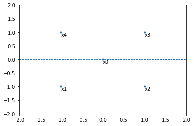
Notice that the distance from \(x_0\) to all other points (\(x_1, x_2, x_3, x_4\)) is the same and we will call it \(d\).
The next step you want to do is to convert it to a 1D space. What happens in the lower dimension is that there is less space to fit all the data from higher dimension. In the graph above we see that there are 5 points and each has its own place. Now let’s take a look at the lower dimension:
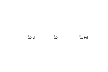
Notice that in the 1D space, there are only two spots for points that are within distance \(d\) from point \(x_0\). What will end up happening is that they will be “crowding” since we have 4 points and only 2 spots available, hence those each of those 1D neighboring points will have 2 points from the 2D space. This is called the crowding problem.
t-SNE efficiently solves this problem by using a more heavy-tailed student t distribution to allow a larger spread between the points hence reducing the “crowding”.
t-Distributed Stochastic Neighbor Embedding (t-SNE) in Python
To continue following this tutorial we will need four Python libraries: pandas, numpy, sklearn, and matplotlib.
If you don’t have them installed, please open “Command Prompt” (on Windows) and install them using the following code:
pip install pandas
pip install numpy
pip install sklearn
pip install matplotlib
Import the required libraries:
import pandas as pd
import numpy as np
import matplotlib.pyplot as plt
from sklearn.datasets import load_wine
from sklearn.preprocessing import StandardScaler
from sklearn.manifold import TSNE
Once the libraries are downloaded, installed, and imported, we can proceed with Python code implementation.
Step 1: Load the dataset
In this tutorial we will use the wine recognition dataset available as a part of sklearn library. This dataset contains 13 features and target being 3 classes of wine. It is the same dataset we used in our Principle Component Analysis article.
Another reason I chose this dataset is because of its shape and because it fits our requirements to show the performance of t-SNE. In addition, you may be already familiar with it from other articles on PyShark.
Let’s store the features into a dataframe with feature names as column names:
wine = load_wine()
df = pd.DataFrame(wine.data, columns=wine.feature_names)
Step 2: Standardize the dataset
To make the dataset more algorithm friendly, we will standardize it:
df = StandardScaler().fit_transform(df)
df=pd.DataFrame(df,columns=wine.feature_names)
Note: this is not necessary, but generally preferred. As well as we explored this dataset in previous articles and found that it’s better to visualize it when it’s standardized, since many algorithms can be affected by the ranges of features being largely different from each other.
Step 3: Applying t-SNE in Python and visualizing the dataset
The sklearn class TSNE() comes with a list of hyper parameters that can be tuned during the application of this technique. We will describe the first 2 of them. However you are encouraged to explore all of them if you are interested in learning about it in depth.
Let’s discuss these 2 hyper parameters:
- n_components : int, optional (default: 2)
This is a parameter for the dimension of the lower space to which you want to convert your dataset to. In our case the value should be 2 since we want to visualize the dataset in a 2 dimensional space. - perplexity : float, optional (default: 30)
This is a parameter for the number of nearest neighbors based on which t-SNE will determine the potential neighbors. Generally, the larger the dataset the larger should be the perplexity value. Below we will show how different perplexity values can affect the results.
First of all, let’s begin with plotting using the t-SNE default values, and setting random_state=0 when creating the instance of t-SNE in Python. You can choose any other integer for random state, we describe its implications in the Appendix.
tsne = TSNE(random_state=0)
tsne_results = tsne.fit_transform(df)

tsne_results=pd.DataFrame(tsne_results, columns=['tsne1', 'tsne2'])

plt.scatter(tsne_results['tsne1'], tsne_results['tsne2'], c=wine.target)
plt.show()
Here we first create the instance of t-SNE in Python and store it as tsne. Next we transform the original dataset to it’s 2 dimensional shape (tsne_results) which comes in the format of numpy array. For the purposes of visualization, we convert it to a pandas dataframe and give names to our columns. Finally we create a scatter plot while the colour label resembles the type of the wine (wine.target).
Here is what we arrive at:
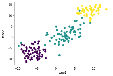
Quite an achievement! We went from 13 dimensions to just 2 and the scatter plot looks great!
t-Distributed Stochastic Neighbor Embedding (t-SNE) Hyperparameter Tuning
This section is for a more advanced reader, but overall it’s just another layer on top of what we already did in the previous section.
As we already know, t-SNE in Python comes with a set of hyperparameters that we can tune. So it doesn’t make sense for us to tune n_components since we always want to have it equal to 2 to work with a 2 dimensional space.
Let’s talk about tuning perplexity and see it’s effects on the visualized output of the transformation.
The sklearn documentation suggests considering a perplexity value between 5 and 50. Seems like this may depend on your dataset and selecting different values can produce significantly different results on a case by case basis.
As an example let’s work with a few values for perplexity: 1, 10, 25, 75.
plt.figure(figsize = (8,4))
plt.subplots_adjust(top = 1.5)

for index, p in enumerate([1, 10, 25, 75]):

    tsne = TSNE(n_components = 2, perplexity = p, random_state=0)
    tsne_results = tsne.fit_transform(df)

    tsne_results=pd.DataFrame(tsne_results, columns=['tsne1', 'tsne2'])

    plt.subplot(2,2,index+1)
    plt.scatter(tsne_results['tsne1'], tsne_results['tsne2'], c=wine.target, s=30)
    plt.title('Perplexity = '+ str(p))
plt.show()
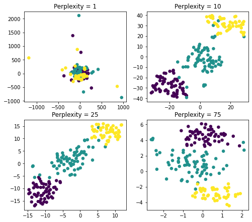
A few important findings that we can conclude from the above visualization:
- Perplexity = 1 : local variations dominate
- Perplexity = 75 : global variations dominate
- Perplexity = 10 or 25 : both in the range recommended and the results seem to be more or less similar
As a result, you can see, perplexity is an important parameter and should be taken into consideration when working with t-SNE to make sure that your visualizations are adjusted correctly.
Additional Information
Recall that in all instances of initializing t-SNE in Python we set the random_state parameter to 0. What exactly does it do?
As its name suggests, random_state is the internal random number generator which decides on indices splitting in the dataset.
Consequently, if it’s not set, then it’s randomly initialized.
Why does it matter for t-SNE? Let’s take a look at the below graphs. Here we create 4 scatterplots with the same parameters except we don’t specify random_state:
plt.figure(figsize=(8, 4))
plt.subplots_adjust(top = 1.5)
tsne = TSNE()
for i in range(4):
    tsne_results = tsne.fit_transform(df)

    tsne_results=pd.DataFrame(tsne_results, columns=['tsne1', 'tsne2'])

    plt.subplot(2,2,int(i)+1)
    plt.scatter(tsne_results['tsne1'], tsne_results['tsne2'], c=wine.target, s = 30)
    plt.title('Run'+str(int(i)+1))

plt.show()
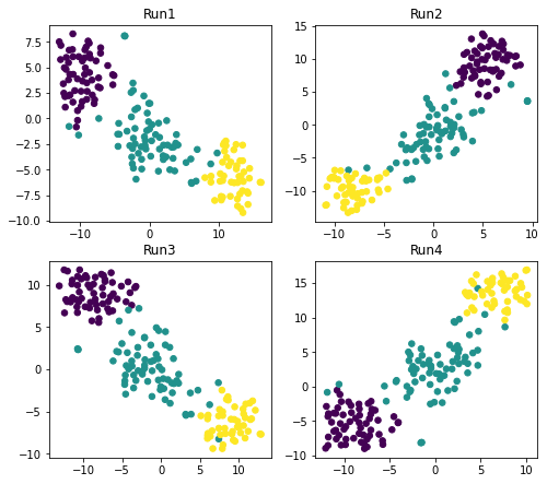
Note: the 4 scatterplots generated by you may differ.
Here we observe that not setting random_seed and executing the code indeed generates 4 different datasets even though other parameters of the model are the same.
Due to the initialization of t-SNE in Python which is random unless you set it otherwise, the above finding occurs. The complexity in case of t-SNE is added because of its cost function and random initialization resulting in different local minima for this function and altering the results in every run.
Conclusion
This article is a walkthrough for application of t-Distributed Stochastic Neighbor Embedding (t-SNE) for visualization of multidimensional datasets in Python.
Furthermore, the next steps you can take to explore the benefits of this technique further is to try an apply this technique to more datasets with advanced hyperparameter tuning and comparing its performance to other dimensionality reduction techniques such as Principal Component Analysis.
Feel free to leave comments below if you have any questions or have suggestions for some edits.