In this article we will explore binomial distribution and binomial test in Python.
Table of contents
- Introduction
- What is a binomial distribution
- Binomial distribution Example
- Create and plot binomial distribution in Python
- What is a binomial test (with Example)
- Binomial test in Python (Example)
- Conclusion
Introduction
To continue following this tutorial we will need the following Python libraries: scipy, numpy, and matplotlib.
If you don’t have it installed, please open “Command Prompt” (on Windows) and install it using the following code:
pip install scipy
pip install numpy
pip install matplotlib
What is a binomial distribution
Binomial distribution is one of the most popular distributions in statistics, along with normal distribution. Binomial distribution is a discrete probability distribution of a number of successes (\(X\)) in a sequence of independent experiments (\(n\)). Each experiment has two possible outcomes: success and failure. Success outcome has a probability \(p\), and failure has probability \((1-p)\).
Note: an individual experiment is also called a Bernoulli trial, an experiment with exactly two possible outcomes. And binomial distribution for one experiment (\(n=1\)) is also a Bernoulli distribution.
In other words, binomial distribution models the probability of observing either success or failure outcome in an independent experiment that is repeated multiple times.
Let’s say probability of success is equal to:
$$p$$
then probability of failure is equal to:
$$q=1-p$$
So the probability of achieving \(k\) successes and \(n-k\) failures is equal to:
$$p^k \times (1-p)^{n-k}$$
And the number of ways to achieve \(k\) successes is calculated as:
$$\frac{n!}{(n-k)! \times k!}$$
Using the above notations we can solve for a probability mass function (total probability of achieving \(k\) successes in \(n\) experiments):
$$f(k;n,p) = Pr(k;n,p) = Pr(X=k) = \frac{n!}{(n-k)! \times k!} p^k (1-p)^{n-k}$$
Note: probability mass function (pmf) – a function that gives the probability that a discrete random variable is exactly equal to some value.
And the formula for the binomial cumulative probability function is:
$$F(k;n,p) = \sum^{x}_{i=0} \frac{n!}{(n-i)! \times i!} p^i (1-p)^{n-i}$$
Binomial distribution Example
You are rolling a single 6-sided die 12 times, and you want to find out the probability of getting 3 as an outcome 5 times. Here, getting 3 is a success outcome, while getting anything else (1, 2, 4, 5, 6) is a failure outcome. Clearly, on each roll, your probability of getting 3 is \(\frac{1}{6}\).
According to the data we have here, rolling a die 12 times, you should get 3 as an outcome 2 times (\(12 \times \frac{1}{6}\)).
Now, how do we actually calculate the probability of observing 3 as an outcome 5 times?
Using the above formula we can easily solve for it. We have an experiment that occurs 12 times (\(n\) = 12), number of outcomes in question is 5 (\(k\) = 5), and probability is \(\frac{1}{6}\) or 0.17 rounded (\(p\) = 0.17).
Plugging into the above equation we get:
$$Pr(5;12,0.17) = Pr(X=5) = \frac{12!}{(12-5)! \times 5!} 0.17^5 (1-0.17)^{12-5} = 0.03$$
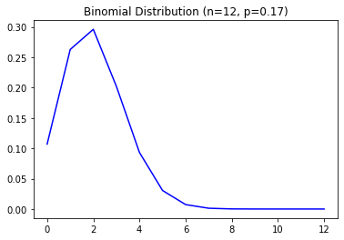
and the binomial distribution for such experiment would look like this:

You can clearly see that observing 3 as an outcome has the highest probability at 2 times, and probability of observing it 5 times is less than 0.05.
Create and plot binomial distribution in Python
Let’s now explore how to create the binomial distribution values and plot it using Python. In this section, we will work with three Python libraries: numpy, matplotlib, and scipy.
We will first import the required modules:
import numpy as np
import matplotlib.pyplot as plt
from scipy.stats import binom
For the data, we will continue with the example from the previous section, where we roll a die 12 times (\(n\) = 12) wherethe probability of observing any number from 1 to 6 is \(\frac{1}{6}\) or 0.17 (\(p\) = 0.17).
Now we will create values for them in Python:
n = 12
p = 0.17
x = np.arange(0, n+1)
where \(x\) is an array of numbers from 0 to 12, representing the number of times any number can be observed.
Using this data we can now calculate the binomial probability mass function. Probability mass function (PMF) is a function that gives the probability that a binomial discrete random variable is exactly equal to some value.
In our example, it will show the number of times from 12 rolls you can observe any number that has probability of 0.17.
Construct PMF:
binomial_pmf = binom.pmf(x, n, p)

print(binomial_pmf)
And you should get an array with 13 values (which are the probabilities for our \(x\) values):
[1.06890008e-01 2.62717609e-01 2.95952970e-01 2.02056244e-01
 9.31162813e-02 3.05152151e-02 7.29178834e-03 1.28014184e-03
 1.63873579e-04 1.49175414e-05 9.16620011e-07 3.41348087e-08
 5.82622237e-10]
Now that we have the binomial probability mass function, we can easily visualize it:
plt.plot(x, binomial_pmf, color='blue')
plt.title(f"Binomial Distribution (n={n}, p={p})")
plt.show()
and you should get:

Now, how about trying to interpret what we see?
The graph shows that if we choose any number from 1 to 6 (die sides) and roll the die 12 times, the highest probability for any of those numbers to be observed is 2 times.
In other words, if I choose number 1 and roll the die 12 times, most likely 1 will show up 2 times.
If you ask, what is the probability that 1 will show up 6 times? By looking at the above graph you can see that it’s slightly more than 0.02 or 2%.
What is a binomial test
Binomial test is a one-sample statistical test of determining whether a dichotomous score comes from a binomial probability distribution.
Using the example from the previous section, let’s reword the question in a way that we can do some hypothesis testing. The following is the situation:
You suspect that a die is biased towards number 3 (three dots) you decided to roll it 12 times (\(n\) = 12) and observed a value of 3 (three dots) 5 times (\(k\) = 5) . You want to understand whether the die is biased towards number 3 or not (recall that expected probability of observing 3 is \(\frac{1}{6}\) or 0.17).
Formulating hypothesis we would have:
$$H_0: \pi \leq \frac{1}{6}$$
$$H_1: \pi > \frac{1}{6}$$
And now calculating the probability:
$$Pr(5;12,0.17) = Pr(X=5) = \frac{12!}{(12-5)! \times 5!} 0.17^5 (1-0.17)^{12-5} = 0.03$$
Here the probability is the \(p\)-value for the significance test. Since 0.03<0.05, we reject the null hypothesis and accept the alternative hypothesis that the die is biased towards number 3.
Binomial test in Python (Example)
Let’s now use Python to do the binomial test for the above example.
It is a very simple few line implementation of .binomtest() function from the scipy library.
Step 1:
Import the function.
from scipy.stats import binomtest
Step 2:
Define the number of successes (\(k\)), define the number of trials (\(n\)), and define the expected probability success (\(p\)).
k=5
n=12
p=0.17
Step 3:
Perform the binomial test in Python.
res = binomtest(k, n, p)
print(res.pvalue)
and we should get:
0.03926688770369119which is the \(p\)-value for the significance test (similar number to the one we got by solving the formula in the previous section).
Note: by default, the test computed is a two-tailed test. If you are working with one-tailed test situation, please refer to the scipy documentation of this function.
Conclusion
In this article we explored binomial distribution and binomial test, as well as how to create and plot binomial distribution in Python, and perform a binomial test in Python.
Feel free to leave comments below if you have any questions or have suggestions for some edits and check out more of my Statistics articles.
