
In this tutorial we will explore continuous and discrete uniform distribution in Python.
Table of contents
- Introduction
- What is a uniform distribution
- Continuous uniform distribution example
- Continuous uniform distribution example in Python
- Discrete uniform distribution example
- Discrete uniform distribution example in Python
Introduction
To continue following this tutorial we will need the following Python libraries: scipy, numpy, and matplotlib.
If you don’t have it installed, please open “Command Prompt” (on Windows) and install it using the following code:
pip install scipy
pip install numpy
pip install matplotlib
What is a uniform distribution
There are two types of uniform distributions:
- Continuous uniform distribution – working with continuous values
- Discrete uniform distribution – working with discrete (finite) values
Continuous uniform distribution
A continuous uniform probability distribution is a distribution with constant probability, meaning that the measures the same probability of being observed.
A continuous uniform distribution is also called a rectangular distribution. Why is that? Let’s explore!
This type of distribution is defined by two parameters:
- \(a\) – the minimum
- \(b\) – the maximum
and is written as: \(U(a, b)\).
The difference between \(b\) and \(a\) is the interval length: \(l=b-a\). Since this is a cumulative distribution, all intervals within the interval length are equally probable (given that those intervals are of the same length).
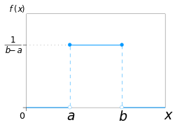
The PDF (probability density function) of a continuous uniform distribution is given by:
$$f(x) = \frac{1}{b-a} \textit{ for } A\leq x \leq B$$
and 0 otherwise.
And the CDF (cumulative distribution function) of a continuous uniform distribution is given by:
$$F(x) = \frac{x-a}{b-a} \textit{ for } A\leq x \leq B$$
with 0 for \(x < a\) and 1 for \(x>b\).
Discrete uniform distribution
A discrete uniform probability distribution, is a distribution with constant probability, meaning that a finite number of values are equally likely to be observed.
This type of distribution is defined by two parameters:
- \(a\) – the minimum
- \(b\) – the maximum
and is written as: \(U(a, b)\).
The difference between \(b\) and \(a\) +1 is the number of observations: The difference between \(b\) and \(a\) is the interval length: \(n=b-a+1\). And all observations are equally probable.
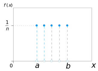
For any \(x \in [a, b]\), the PMF (probability mass function) of a discrete uniform distribution is given by:
$$f(x) = \frac{1}{b-a+1} = \frac{1}{n}$$
And for any \(x \in [a, b]\), the CDF (cumulative distribution function) of a discrete uniform distribution is given by:
$$F(x) = P(X\leq x) = \frac{x-a+1}{b-a+1} = \frac{x-a+1}{n}$$
Continuous uniform distribution example
Let’s consider an example: you live in an apartment building that has 10 floors and just came home. You entered the lobby and about to press the elevator button. You know that it can take anywhere between 0 and 20 seconds for you to wait for the elevator, where it takes 0 seconds if the elevator is on the first floor (no wait), and it takes 20 seconds if the elevator is on the tenth floor (maximum wait). This would be an example of a continuous uniform distribution, since the wait time can take any value with the same probability and is continuous because the elevator can be anywhere in the building between first and tenth floor (for example, between fifth and sixth floor).
Here we have the minimum value \(a = 0\), and the maximum value \(b = 20\).
Continuous uniform distribution PDF
Knowing the values of \(a\) and \(b\), we can easily compute the continuous uniform distribution PDF:
$$f(x)=\frac{1}{20-0} = \frac{1}{20} = 0.05$$
Using the \(f(x)\) formula and given parameters we can create the following visualization of continuous uniform PDF:
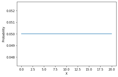
So what does this really tell us in the context of a continuous uniform distribution? Let’s take two 1 second intervals anywhere on the interval [0, 20]. For example from 1 to 2 (\(i_1 = [1, 2]\)) and from 15 to 16 (\(i_2 = [15, 16]\)). Important to note that both of these intervals are of the same length equal to 1. Using the PMF result, we can say that these intervals are equally likely to occur with probability 0.05. In other words, it is as likely for the elevator to arrive between 1 and 2 seconds, as it is to arrive between 15 and 16 seconds (with probability 0.05).
Continuous uniform distribution CDF
Now let’s consider an addition to the example in this section. You are still in the apartment building waiting for the elevator, but now you want to find out what is the probability that it will take the elevator 6 seconds or less to arrive after you press the button.
Using continuous distribution CDF formula from this section we can solve for:
$$F(6) = P(X\leq 6) = \frac{6-0}{20} = \frac{6}{20} = 0.3$$
We observe that the probability that it will take the elevator 6 seconds or less (anywhere between 0 and 6) to arrive is 0.3.
Using \(F(x)\) formula and given parameters we can create the following visualization of continuous uniform CDF:
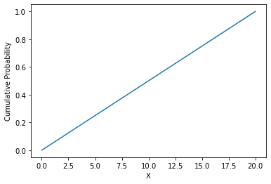
And we observe a linear relationship between cumulative probability and random variable \(X\), where the function is monotonically increasing at the rate \(f(x)\) (in our case \(f(x)=0.05\)).
Continuous uniform distribution example in Python
In one of the previous sections we computed continuous uniform distribution probability density function by hand. In this section, we will reproduce the same results using Python.
We will begin with importing the required dependencies:
import numpy as np
import matplotlib.pyplot as plt
from scipy.stats import uniform
Next, we will create a continuous array of values between 0 and 20 (minimum and maximum wait times). Mathematically, there is an infinitely large number of values, so for purposes of this example we will create 4,000 values in range between 0 and 20. We will also print the first 3 of them just to take a look.
a=0
b=20
size=4000

x = np.linspace(a, b, size)

print(x[:3])
And you should get:
[0. 0.00500125 0.0100025 ]And now we will have to create a uniform continuous random variable using scipy.stats.uniform:
continuous_uniform_distribution = uniform(loc=a, scale=b)
In the following sections we will focus on calculating the PDF and CDF using Python.
Continuous uniform distribution PDF in Python
In order to calculate the cumulative uniform distribution PDF using Python, we will use the .pdf() method of the scipy.stats.uniform generator:
continuous_uniform_pdf = continuous_uniform_distribution.pdf(x)

print(continuous_uniform_pdf)
And you should get:
[0.05 0.05 0.05 ... 0.05 0.05 0.05]So now we found the probabilities for each value are the same and equal to 0.05, which is exactly the same as we calculated by hand.
Plot continuous uniform distribution PDF using Python
Using matplotlib library, we can easily plot the continuous uniform distribution PDF using Python:
plt.plot(x, continuous_uniform_pdf)
plt.xlabel('X')
plt.ylabel('Probability')
plt.show()
And you should get:
Continuous uniform distribution CDF in Python
In order to calculate the continuous uniform distribution CDF using Python, we will use the .cdf() method of the scipy.stats.uniform generator:
continuous_uniform_cdf = continuous_uniform_distribution.cdf(x)
Since we will have 4,000 values, if we want to double check the correctness of the calculations that we did by hand, you will need to find the cumulative probability associated with the value equal to 6. It is indeed around 0.3.
Plot continuous uniform distribution CDF using Python
Using matplotlib library, we can easily plot the continuous uniform distribution CDF using Python:
plt.plot(x, continuous_uniform_cdf)
plt.xlabel('X')
plt.ylabel('Cumulative Probability')
plt.show()
And you should get:

Discrete uniform distribution example
Let’s consider an example (and this is the one most us did ourselves): rolling the dice. Basically, the possible outcomes of rolling a single 6-sided die follow the discrete uniform distribution.
Why is that? It’s because you can only have 1 outcome from 6 possible outcomes (you can get either: 1, 2, 3, 4, 5, or 6). The number of possible outcomes if finite and each outcome has an equal probability of being observed, which is \(\frac{1}{6}\).
Discrete uniform distribution PMF
Knowing the number of all possible outcomes \(n\), we can easily compute the discrete uniform distribution PMF:
$$f(x)=\frac{1}{6} = 0.16$$
Using the \(f(x)\) formula and given parameters we can create the following visualization of discrete uniform PMF:

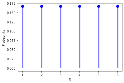
In this example, each side of the die has an equal opportunity of being observed equal to 0.16.
Discrete uniform distribution CDF
Now let’s consider an addition to this example. You are rolling the same 6-sided die and now want to find out the probability of you observing outcome that is equal to or less than 2 (meaning either 1 or 2).
Knowing the number of all possible outcomes \(n\), we can easily compute the discrete uniform distribution CDF:
$$F(2)=\frac{2-1+1}{6-1+1} = \frac{2}{6} = 0.33$$
This tells us that if we roll a 6-sided die, the probability of observing a value less than or equal to 2 is 0.33.
Using the \(F(x)\) formula and given parameters we can create the following visualization of discrete uniform CDF:
And we observe a step-wise relationship since we have discrete values as possible outcomes.
Discrete uniform distribution example in Python
In one of the previous sections we computed continuous uniform distribution cumulative distribution function by hand. In this section, we will reproduce the same results using Python.
We will begin with importing the required dependencies:
import numpy as np
import matplotlib.pyplot as plt
from scipy.stats import randint
Next, we will create an array of values between 1 and 6 (smallest and largest die values), and print them to take a look.
a=1
b=6

x = np.arange(a, b+1)

print(x)
And you should get:
[1 2 3 4 5 6]And now we will have to create a uniform continuous random variable using scipy.stats.randint:
discrete_uniform_distribution = randint(a, b+1)
In the following sections we will focus on calculating the PMF and CDF using Python.
Discrete uniform distribution PMF in Python
In order to calculate the discrete uniform distribution PMF using Python, we will use the .pmf() method of the scipy.stats.randint generator:
discrete_uniform_pmf = discrete_uniform_distribution.pmf(x)

print(discrete_uniform_pmf)
You should get:
[0.16666667 0.16666667 0.16666667 0.16666667 0.16666667 0.16666667]Which is exactly the 0.16 value that we calculated by hand.
Plot discrete uniform distribution PMF using Python
Using matplotlib library, we can easily plot the discrete uniform distribution PMF using Python:
plt.plot(x, discrete_uniform_pmf, 'bo', ms=8)
plt.vlines(x, 0, discrete_uniform_pmf, colors='b', lw=5, alpha=0.5)
plt.xlabel('X')
plt.ylabel('Probability')
plt.show()
And you should get:
Discrete uniform distribution CDF in Python
In order to calculate the discrete uniform distribution PMF using Python, we will use the .cdf() method of the scipy.stats.randint generator:
discrete_uniform_cdf = discrete_uniform_distribution.cdf(x)

print(discrete_uniform_cdf)
And you should get:
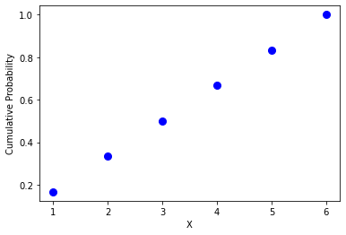
[0.16666667 0.33333333 0.5 0.66666667 0.83333333 1. ]We see here that the second value in the array is 0.33 which is exactly the same as we calculated by hand.
Plot discrete uniform distribution CDF using Python
Using matplotlib library, we can easily plot the discrete uniform distribution CDF using Python:
plt.plot(x, discrete_uniform_cdf, 'bo', ms=8)
plt.xlabel('X')
plt.ylabel('Cumulative Probability')
plt.show()
And you should get:

Conclusion
In this article we explored cumulative uniform distribution and discrete uniform distribution, as well as how to create and plot them in Python.
Feel free to leave comments below if you have any questions or have suggestions for some edits and check out more of my Statistics articles.