
In this article we will explore Poisson distribution and Poisson process in Python.
Table of contents
- Introduction
- What is a Poisson process
- What is a Poisson distribution
- Poisson distribution example
- Poisson distribution example in Python
- Conclusion
Introduction
To continue following this tutorial we will need the following Python libraries: scipy, numpy, and matplotlib.
If you don’t have it installed, please open “Command Prompt” (on Windows) and install it using the following code:
pip install scipy
pip install numpy
pip install matplotlib
What is a Poisson process
A Poisson point process (or simply, Poisson process) is a collection of points randomly located in mathematical space.
Due to its several properties, the Poisson process is often defined on a real line, where it can be considered a random (stochastic) process in one dimension. This further allows to build mathematical systems and study certain events that appear in a random manner.
One of its important properties is that each point of the process is stochastically independent from other points in the process.
As an example we can think of an example where such process can be observed in real life. Suppose you are studying the historical frequencies of hurricanes. This indeed is a random process, since the number of hurricanes this year is independent of the number of hurricanes las year and so on. However, over time you may be observing some trends, average frequency, and more.
Mathematically speaking, in this case, the point process depends on something that might be some constant, such as average rate (average number of customers calling, for example).
A Poisson process is defined by a Poisson distribution.
What is a Poisson distribution?
A Poisson distribution is a discrete probability distribution of a number of events occurring in a fixed interval of time given two conditions:
- Events occur with some constant mean rate.
- Events are independent of each other and independent of time.
To put this in some context, consider our example of frequencies of hurricanes from the previous section.
Assume that when we have data on observing hurricanes over a period of 20 years. We find that the average number of hurricanes per year is 7. Each year is independent of previous years, which means that if we observed 8 hurricanes this year, it doesn’t mean we will observe 8 next year.
The PMF (probability mass function) of a Poisson distribution is given by:
$$p(k, \lambda) = \frac{\lambda^{k}e^{-\lambda}}{k!}$$
where:
- \(\lambda\) is a real positive number given by \(\lambda = E(X) = \mu\)
- \(k\) is the number of occurrences
- \(e = 2.71828\)
The \(Pr(X=k)\) can be read as: Poisson probability of k events in an interval.
And the CDF (cumulative distribution function) of a Poisson distribution is given by:
$$F(k, \lambda) = \sum^{k}_{i=0} \frac{\lambda^{i}e^{-\lambda}}{i!}$$
Poisson distribution example
Now that we know some formulas to work with, let’s go through an example in detail.
Recall the hurricanes data we mentioned in the previous sections. We know that the historical frequency of hurricanes is 7 per year (which is the rate, \(\mu\), and this forms our \(\lambda\) value (since \(\lambda=\mu\)):
$$\lambda = 7$$
The question we can have is what is the probability of observing exactly 5 hurricanes this year? And this forms our \(k\) value:
$$k = 5$$
Using the formula from the previous section, we can calculate the Poisson probability:
$$p(5, 7) = \frac{(7^{5})(e^{-7})}{5!} = 0.12772 \approx 12.77\%$$
Therefore, the probability of observing exactly 5 hurricanes next year is equal to 12.77%.
Naturally, we are curious about the probabilities of other frequencies.
Poisson PMF (probability mass function)
Consider the table below which shows the Poisson probability of hurricane frequencies (0-15):
| \(k\) | \(p(k, \lambda)\) | % |
| 0 | 0.00091 | 0.09% |
| 1 | 0.00638 | 0.64% |
| 2 | 0.02234 | 2.23% |
| 3 | 0.05213 | 5.21% |
| 4 | 0.09123 | 9.12% |
| 5 | 0.12772 | 12.77% |
| 6 | 0.14900 | 14.9% |
| 7 | 0.14900 | 14.9% |
| 8 | 0.13038 | 13.04% |
| 9 | 0.10140 | 10.14% |
| 10 | 0.07098 | 7.01% |
| 11 | 0.04517 | 4.52% |
| 12 | 0.02635 | 2.64% |
| 13 | 0.01419 | 1.42% |
| 14 | 0.00709 | 0.71% |
| 15 | 0.00331 | 0.33% |
| 16 | 0.00145 | 0.15% |
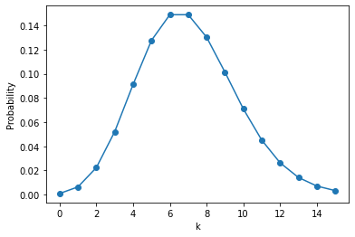
Using the above table we can create the following visualization of the Poisson probability mass function for this example:
Poisson CDF (cumulative distribution function)
Consider the table below which shows the Poisson cumulative probability of hurricane frequencies (0-15):
| \(k\) | \(F(k, \lambda)\) | % |
| 0 | 0.00091 | 0.09% |
| 1 | 0.00730 | 0.73% |
| 2 | 0.02964 | 2.96% |
| 3 | 0.08177 | 8.18% |
| 4 | 0.17299 | 17.3% |
| 5 | 0.30071 | 30.07% |
| 6 | 0.44971 | 44.97% |
| 7 | 0.59871 | 59.87% |
| 8 | 0.72909 | 72.91% |
| 9 | 0.83050 | 83.05% |
| 10 | 0.90148 | 90.15% |
| 11 | 0.94665 | 94.67% |
| 12 | 0.97300 | 97.3% |
| 13 | 0.98719 | 98.72% |
| 14 | 0.99428 | 99.43% |
| 15 | 0.99759 | 99.76% |
| 16 | 0.99904 | 99.9% |
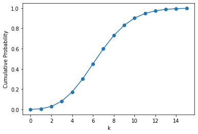
Using the above table we can create the following visualization of the Poisson cumulative distribution function for this example:
The table also allows us to answer some interesting questions.
For example, what if we wanted to find out the probability of seeing up to 5 hurricanes (mathematically: \(k\leq5\)), we can see that it’s \(0.30071\) or \(30.07\%\).
On the other hand, we can be interested in probability of observing more than 5 hurricanes (mathematically: \(k>5\)), which would be \(1-p(5,7) = 1-0.30071 = 0.69929\) or \(69.93\%\).
Poisson distribution example in Python
In the previous section we computed probability mass function and cumulative distribution function by hand. In this section, we will reproduce the same results using Python.
We will begin with importing the required dependencies:
import numpy as np
import matplotlib.pyplot as plt
from scipy.stats import poisson
Next we will need an array of the \(k\) values for which we will compute the Poisson PMF. In the previous section, we calculated it for 16 values of \(k\) from 0 to 16, so let’s create an array with these values:
k = np.arange(0, 17)

print(k)
You should get:
[ 0 1 2 3 4 5 6 7 8 9 10 11 12 13 14 15 16]In the following sections we will focus on calculating the PMF and CDF using Python.
Poisson PMF (probability mass function) in Python
In order to calculate the Poisson PMF using Python, we will use the .pmf() method of the scipy.poisson generator. It will need two parameters:
- \(k\) value (the k array that we created)
- \(\mu\) value (which we will set to 7 as in our example)
And now we can create an array with Poisson probability values:
pmf = poisson.pmf(k, mu=7)
pmf = np.round(pmf, 5)

print(pmf)
And you should get:
[0.00091 0.00638 0.02234 0.05213 0.09123 0.12772 0.149 0.149 0.13038 0.1014 0.07098 0.04517 0.02635 0.01419 0.00709 0.00331 0.00145]Note:
If you want to print it in a nicer way with each \(k\) value and the corresponding probability:
for val, prob in zip(k,pmf):
    print(f"k-value {val} has probability = {prob}")
And you should get:
k-value 0 has probability = 0.00091
k-value 1 has probability = 0.00638
k-value 2 has probability = 0.02234
k-value 3 has probability = 0.05213
k-value 4 has probability = 0.09123
k-value 5 has probability = 0.12772
k-value 6 has probability = 0.149
k-value 7 has probability = 0.149
k-value 8 has probability = 0.13038
k-value 9 has probability = 0.1014
k-value 10 has probability = 0.07098
k-value 11 has probability = 0.04517
k-value 12 has probability = 0.02635
k-value 13 has probability = 0.01419
k-value 14 has probability = 0.00709
k-value 15 has probability = 0.00331
k-value 16 has probability = 0.00145
which is exactly the same as we saw in the example where we calculated probabilities by hand.
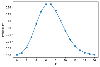
Plot Poisson PMF using Python
We will need the k values array that we created earlier as well as the pmf values array in this step.
Using matplotlib library, we can easily plot the Poisson PMF using Python:
plt.plot(k, pmf, marker='o')
plt.xlabel('k')
plt.ylabel('Probability')

plt.show()
And you should get:
Poisson CDF (cumulative distribution function) in Python
In order to calculate the Poisson CDF using Python, we will use the .cdf() method of the scipy.poisson generator. It will need two parameters:
- \(k\) value (the k array that we created)
- \(\mu\) value (which we will set to 7 as in our example)
And now we can create an array with Poisson cumulative probability values:
cdf = poisson.cdf(k, mu=7)
cdf = np.round(cdf, 3)

print(cdf)
And you should get:
[0.001 0.007 0.03  0.082 0.173 0.301 0.45  0.599 0.729 0.83  0.901 0.947
  0.973 0.987 0.994 0.998 0.999]
Note:
If you want to print it in a nicer way with each \(k\) value and the corresponding cumulative probability:
for val, prob in zip(k,cdf):
    print(f"k-value {val} has probability = {prob}")
And you should get:
k-value 0 has probability = 0.001
k-value 1 has probability = 0.007
k-value 2 has probability = 0.03
k-value 3 has probability = 0.082
k-value 4 has probability = 0.173
k-value 5 has probability = 0.301
k-value 6 has probability = 0.45
k-value 7 has probability = 0.599
k-value 8 has probability = 0.729
k-value 9 has probability = 0.83
k-value 10 has probability = 0.901
k-value 11 has probability = 0.947
k-value 12 has probability = 0.973
k-value 13 has probability = 0.987
k-value 14 has probability = 0.994
k-value 15 has probability = 0.998
k-value 16 has probability = 0.999
which is exactly the same as we saw in the example where we calculated cumulative probabilities by hand.
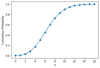
Plot Poisson CDF using Python
We will need the k values array that we created earlier as well as the pmf values array in this step.
Using matplotlib library, we can easily plot the Poisson PMF using Python:
plt.plot(k, cdf, marker='o')
plt.xlabel('k')
plt.ylabel('Cumulative Probability')

plt.show()
And you should get:
Conclusion
In this article we explored Poisson distribution and Poisson process, as well as how to create and plot Poisson distribution in Python.
Feel free to leave comments below if you have any questions or have suggestions for some edits and check out more of my Statistics articles.