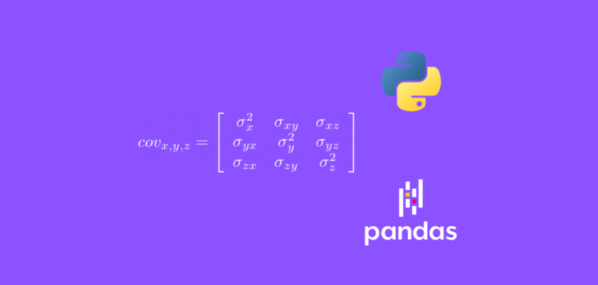
Compute Variance-Covariance Matrix using Python

In this article we will discuss how to compute a variance-covariance matrix using Python.

Table of Contents

Introduction

Variance-covariance matrix explained
Variance-covariance matrix example
Create a sample DataFrame

Compute variance-covariance matrix using Python
Conclusion

Introduction

A variance-covariance matrix is a square matrix (has the same number of rows and columns) that gives the covariance between each pair of elements available in the data.

Covariance measures the extent to which to variables move in the same direction.

In the variance-covariance matrix, variances of variables appear on the diagonal and covariances of variables are all other elements of the matrix.

To continue following this tutorial we will need the following Python library: pandas.

If you don’t have them installed, please open “Command Prompt” (on Windows) and install them using the following code:


pip install pandas

Books I recommend:

Python Crash Course

[the_ad id=”2889″]

[the_ad id=”2891″]

[the_ad id=”2892″]

[the_ad id=’2894′]

Variance-Covariance Matrix Explained

A covariance matrix is:

Symmetric
The square matrix is equal to its transpose: $ A = A^T $.
Positive semi-definite

With main diagonal containing the variances (covariances of variables on themselves)

$$
cov_{x,y,z} = \left[ \begin{array}{ccc}
cov_{x,x} & cov_{x,y} & cov_{x,z} \\
cov_{y,x} & cov_{y,y} & cov_{y,z} \\
cov_{z,x} & cov_{z,y} & cov_{z,z}
\end{array} \right]
= \left[ \begin{array}{ccc}
\sigma^2_{x} & \sigma_{xy} & \sigma_{xz} \\
\sigma_{yx} & \sigma^2_{y} & \sigma_{yz} \\
\sigma_{zx} & \sigma_{zy} & \sigma^2_{z}
\end{array} \right]
$$

where each covariance can be computed by the following formula (replacing x, y, z values):

$$
cov_{x,y} = E[(X – E[X])(Y – E[Y])] = \frac{\sum(x_i – \bar{x})(y_i – \bar{y})}{N-1}
$$

Variance-Covariance Matrix Example

First, let’s consider some sample data to work with:

Age	Experience	Salary
25	2	2000
32	6	3000
37	9	3500

Alternatively, the above table can be represented as a matrix:

$$A = \begin{bmatrix} 25 & 2 & 2000 \\ 32 & 6 & 3000 \\ 37 & 9 & 3500 \end{bmatrix}$$

Then the covariance matrix of $A$ will look like:

$$
cov_{a,e,s} = \left[ \begin{array}{ccc}
cov_{a,a} & cov_{a,e} & cov_{a,s} \\
cov_{e,a} & cov_{e,e} & cov_{e,s} \\
cov_{s,a} & cov_{s,e} & cov_{s,s}
\end{array} \right]
$$

where $a$, $e$, $s$ are Age, Experience, and Salary respectively.

Finally, using the covariance formula:

$$
cov_{x,y} = E[(X – E[X])(Y – E[Y])] = \frac{\sum(x_i – \bar{x})(y_i – \bar{y})}{N-1}
$$

we can calculate the covariance between each pair and populate the variance-covariance matrix:

$ cov_{a,a} = \frac{\sum(Age_i – \bar{Age})(Age_i – \bar{Age})}{N-1} = \\ = \frac{(25-31.33)(25-31.33) + (32-31.33)(32-31.33) + (37-31.33)(37-31.33)}{3-1} = \\ = \frac{40.0689 + 0.4489 + 32.1489}{2} \approx 36.33 $

$ cov_{a,e} = cov_{e,a} = \frac{\sum(Age_i – \bar{Age})(Experience_i – \bar{Experience})}{N-1} = \\
= \frac{(25-31.33)(2-5.66) + (32-31.33)(6-5.66) + (37-31.33)(9-5.66)}{3-1} = \\ = \frac{23.1678 + 0.2278 + 18.9378}{2} \approx 21.17 $

$ cov_{a,s} = cov_{s,a} = \frac{\sum(Age_i – \bar{Age})(Salary_i – \bar{Salary})}{N-1} = \\
= \frac{(25-31.33)(2,000-2,833.33) + (32-31.33)(3,000-2,833.33) + (37-31.33)(3,500-2,833.33)}{3-1} = \\ = \frac{5,274.9789 + 111.6689 + 3,780.0189}{2} \approx 4,583.33 $

$ cov_{e,e} = \frac{\sum(Experience_i – \bar{Experience})(Experience_i – \bar{Experience})}{N-1} = \\
= \frac{(2-5.67)(2-5.67) + (6-5.67)(6-5.67) + (9-5.67)(9-5.67)}{3-1} = \\ = \frac{13.4689 + 0.1089 + 11.0889}{2} \approx 12.33 $

$ cov_{e,s} = cov_{s,e} = \frac{\sum(Experience_i – \bar{Experience})(Salary_i – \bar{Salary})}{N-1} = \\
= \frac{(2-5.67)(2,000-2,833.33) + (6-5.67)(3,000-2,833.33) + (9-5.67)(3,500-2,833.33)}{3-1} = \\ = \frac{3,058.3211 + 55.0011 + 2,220.0111}{2} \approx 2,666.67 $

$ cov_{s,s} = \frac{\sum(Salary_i – \bar{Salary})(Salary_i – \bar{Salary})}{N-1} = \\
= \frac{(2,000-2,833.33)(2,000-2,833.33) + (3,000-2,833.33)(3,000-2,833.33) + (3,500-2,833.33)(3,500-2,833.33)}{3-1} = \\ = \frac{694,438.8889 + 27,778.8889 + 444,448.889}{2} \approx 583,333.33 $

Using the calculated covariance values, we can now populate the variance-covariance matrix:

$$
cov_{a,e,s} = \left[ \begin{array}{ccc}
36.33 & 21.17 & 4,583.33 \\
21.17 & 12.33 & 2,666.67 \\
4,583.33 & 2,666.67 & 583,333.33
\end{array} \right]
$$

Create a sample DataFrame

Let’s create a sample Pandas DataFrame with three variables: Age, Experience, Salary with a few observations for each:


import pandas as pd

df = pd.DataFrame(
    {'Age': [25, 32, 37],
    'Experience': [2, 6, 9],
    'Salary': [2000, 3000, 3500]}
    )

print(df)

And we get:

   Age  Experience  Salary
0   25           2    2000
1   32           6    3000
2   37           9    3500

Using the .cov() method of the Pandas DataFrame we are are able to compute the variance-covariance matrix using Python:


cov_matrix = df.cov()

print(cov_matrix)

And we get:

                    Age   Experience         Salary
Age           36.333333    21.166667    4583.333333
Experience    21.166667    12.333333    2666.666667
Salary      4583.333333  2666.666667  583333.333333

Conclusion

In this article we discussed how to compute a variance-covariance matrix using Python.

Feel free to leave comments below if you have any questions or have suggestions for some edits and check out more of my Statistics articles.

Compute Variance-Covariance Matrix using Python

Introduction

Variance-Covariance Matrix Explained

Variance-Covariance Matrix Example

Create a sample DataFrame