In this tutorial we will explore the Davies-Bouldin index and its application to K-Means clustering evaluation in Python.
[the_ad id=”3031″]Table of Contents
Introduction
The Davies-Bouldin index (DBI) is one of the clustering algorithms evaluation measures. It is most commonly used to evaluate the goodness of split by a K-Means clustering algorithm for a given number of clusters.
We have previously discussed the Dunn index and Calinski-Harabasz index, and Davies-Bouldin index is yet another metric to evaluate the performance of clustering.
What is Davies-Bouldin index?
Davies-Bouldin index is calculated as the average similarity of each cluster with a cluster most similar to it.
How do you interpret Davies-Bouldin index?
The the Davies-Bouldin index (lower the average similarity) is, the better the clusters are separated and the better is the result of the clustering performed.
In the next section the process of calculating the DBI is described in detail with a few examples.
To continue following this tutorial we will need the following Python libraries: sklearn and matplotlib.
If you don’t have it installed, please open “Command Prompt” (on Windows) and install it using the following code:
pip install sklearn
pip install matplotlib
Books I recommend:
- Python Crash Course
- Automate the Boring Stuff with Python
- Beyond the Basic Stuff with Python
- Serious Python
Davies-Bouldin Index Explained
The research on cluster separation using this measure was published back in 1979. The material presented describes a measurement of similarity between clusters as a function of intra-cluster dispersion and separation between the clusters.
In this part we will go through each step of the calculations and provide meaningful illustrative examples to help better understand the formulas.
Step 1: Calculate intra-cluster dispersion
Consider the following equation defined by Davies, D., & Bouldin, D. (1979) that calculates the dispersion of cluster \(i\):
$$S_i = \Bigg\{\frac{1}{T_i} \sum_{j=1}^{T_i} |X_j – A_i|^q \Bigg\}^\frac{1}{q}$$
where:
- \(i\) : particular identified cluster
- \(T_i\) : number of vectors (observations) in cluster \(i\)
- \(T_i\) : number of vectors (observations) in cluster \(i\)
- \(X_j\) : \(j\)-th vector (observation) in cluster \(i\)
- \(A_i\) : centroid of cluster \(i\)
Basically, to get the intra-cluster dispersion, we calculate the average distance between each observation within the cluster and its centroid.
Note: usually the value \(q\) is set to 2 (\(q = 2\)), which calculates the Euclidean distance between the centroid of the cluster and each individual cluster vector (observation).
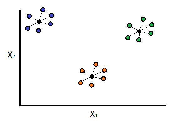
Assume the K-Means clustering that was performed on some dataset generated three clusters. Using the above formula, the intra-cluster dispersion would be calculated for each of the clusters and we will have values for \(S_1\), \(S_2\), and \(S_3\).
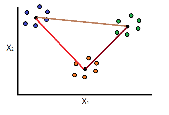
Step 2: Calculate separation measure
Consider the following equation defined by Davies, D., & Bouldin, D. (1979) that calculates the separation between clusters \(i\) and \(j\):
$$M_{ij} = \Bigg\{\sum_{k=1}^{N} |a_{ki} – a_{kj}|^p \Bigg\}^\frac{1}{p}$$
where:
- \(a_{ki}\) : \(k\)-th component of \(n\)-dimensional centroid \(A_i\)
- \(a_{kj}\) : \(k\)-th component of \(n\)-dimensional centroid \(A_j\)
- \(N\) : total number of clusters
The above formula can also be written as:
$$M_{ij} = \Bigg\{\sum_{k=1}^{N} |a_{ki} – a_{kj}|^p \Bigg\}^\frac{1}{p} = ||A_i – A_j||_p$$
Note: when \(p\) is set to 2 (\(p = 2\)), the above formula calculates the Euclidean distance between the centroids of clusters \(i\) and \(j\).
Continue to assume that we are working with three clusters. Using the above formula, we will compute the separation measure for each possible combination of two clusters: \(M_{11}\), \(M_{12}\), \(M_{13}\), \(M_{21}\), \(M_{22}\), \(M_{23}\), \(M_{31}\), \(M_{32}\), and \(M_{33}\).
Of course we also have \(M_{12} = M_{21}\), \(M_{13} = M_{31}\), and \(M_{23} = M_{32}\).
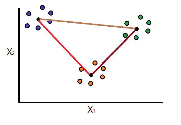
Step 3: Calculate similarity between clusters
Consider the following equation defined by Davies, D., & Bouldin, D. (1979) that calculates the similarity between clusters \(i\) and \(j\):
$$R_{ij} = \frac{S_i + S_j}{M_{ij}}$$
where:
- \(S_i\) : intra-cluster dispersion of cluster \(i\)
- \(S_j\) : intra-cluster dispersion of cluster \(j\)
- \(M_{ij}\) : distance between centroids of clusters \(i\) and \(j\)
Basically here we are computing similarity between clusters as a sum of two intra-cluster dispersions divided by the separation measure. The larger \(R_{ij}\) is, the more similar clusters \(i\) and \(j\) are. You can probably already tell that the best possible case is when these number overall are as low as possible.
Similarly to the logic in Step 2, continue to assume that we are working with three clusters. Using the above formula, we will compute the similarity for each possible combination of two clusters: \(R_{11}\), \(R_{12}\), \(R_{13}\), \(R_{21}\), \(R_{22}\), \(R_{23}\), \(R_{31}\), \(R_{32}\), and \(R_{33}\).
Here, \(R_{11}\) = \(R_{22}\) = \(R_{12}\) are the similarities of each cluster to itself. And we also have \(R_{12} = R_{21}\), \(R_{13} = R_{31}\), and \(R_{23} = R_{32}\).
Step 4: Find most similar cluster for each cluster \(i\)
Davies, D., & Bouldin, D. (1979) define:
$$R_i \equiv maximum(R_{ij})$$
having: \(i \neq j \)
For each cluster \(i\) we find the highest ratio from all \(R_{ij}\) calculated.
For example, for cluster \(i = 1\), we calculated \(R_{11}\), \(R_{12}\), and \(R_{13}\). Continue with \(R_{12}\) and \(R_{13}\) (since \(R_{11}\) doesn’t satisfy the constraint \(i \neq j \), and it makes no sense to compare the cluster with itself).
Now, having \(R_{12}\) (which is similarity between clusters 1 and 2) and \(R_{13}\) (which is similarity between clusters 1 and 3). From these two measures, we would pick the largest one and refer to the maximum measure as \(R_{1}\). Following the same logic we will find \(R_{2}\) and \(R_{3}\).
Step 5: Calculate Davies-Bouldin Index
Calculate the Davies-Bouldin index as:
$$\bar{R} = \frac{1}{N}\sum_{i=1}^{N}R_i$$
which is simply the average of the similarity measures of each cluster with a cluster most similar to it.
Note:
The best choice for clusters is where the average similarity is minimized, therefore a smaller \(\bar{R}\) represents better defined clusters.
Note:
In most of the resources you will see Davies-Bouldin index formula written as:
$$\bar{D} = \frac{1}{N}\sum_{i=1}^{N}D_i$$
where \(D\) is the same as \(R\) in our example.
[the_ad id=”3031″]Davies-Bouldin Index Example in Python
In this section we will go through an example of calculating the Davis-Bouldin index for a K-Means clustering algorithm in Python.
First, import the required dependencies:
from sklearn.datasets import load_iris
from sklearn.cluster import KMeans
from sklearn.metrics import davies_bouldin_score
import matplotlib.pyplot as plt
You can use any data with the code below. For simplicity we will use the built in Iris dataset, specifically the first two features: “sepal width” and “sepal length”:
iris = load_iris()
X = iris.data[:, :2]
Let’s start with K-Means target of 3 clusters:
kmeans = KMeans(n_clusters=3, random_state=30)
labels = kmeans.fit_predict(X)
And check the Davies-Bouldin index for the above results:
db_index = davies_bouldin_score(X, labels)
print(db_index)
You should see the resulting score: 0.7675522686571647 or approximately 0.77.
To put in perspective how the clusters look , let’s visualize them:
unique_labels = list(set(labels))
colors = ['red', 'orange', 'grey']

for i in unique_labels:
    filtered_label = X[labels == i]
    plt.scatter(filtered_label[:,0],
                filtered_label[:,1],
                color = colors[i],
                edgecolor='k')

plt.xlabel('Sepal length')
plt.ylabel('Sepal width')
plt.show()
We should see the following original 3 clusters:
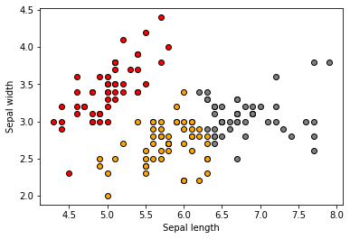
Looks like some clusters are better defined than others.
So far we only computed the Davies-Bouldin index for 3 clusters. This measure can be used similarly to the Elbow Method, to help identify an optimal number of clusters.
We can run the calculation for any number of clusters greater or equal to 2. Let’s try up to 10 clusters:
results = {}

for i in range(2,11):
    kmeans = KMeans(n_clusters=i, random_state=30)
    labels = kmeans.fit_predict(X)
    db_index = davies_bouldin_score(X, labels)
    results.update({i: db_index})
and visualize it:
plt.plot(list(results.keys()), list(results.values()))
plt.xlabel("Number of clusters")
plt.ylabel("Davies-Boulding Index")
plt.show()
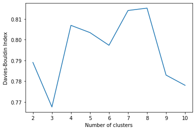
While in this example the measures are very close to each other, we can still observe that choosing 3 clusters minimizes the similarity measure.
[the_ad id=”3031″]Conclusion
In this article we discussed how to calculate the Davies-Bouldin index for clustering evaluation in Python using sklearn library.
Feel free to leave comments below if you have any questions or have suggestions for some edits and check out more of my Python Programming articles.
References:
Davies, D., & Bouldin, D. (1979). A Cluster Separation Measure. IEEE Transactions on Pattern Analysis and Machine Intelligence, PAMI-1(2), 224–227. https://doi.org/10.1109/TPAMI.1979.4766909