In this article we will discuss cosine similarity with examples of its application to product matching in Python.
Table of Contents
Introduction
A lot of interesting cases and projects in the recommendation engines field heavily relies on correctly identifying similarity between pairs of items and/or users.
There are several approaches to quantifying similarity which have the same goal yet differ in the approach and mathematical formulation.
In this article we will explore one of these quantification methods which is cosine similarity. And we will extend the theory learnt by applying it to the sample data trying to solve for user similarity.
The concepts learnt in this article can then be applied to a variety of projects: documents matching, recommendation engines, and so on.
Cosine similarity overview
Cosine similarity is a measure of similarity between two non-zero vectors. It is calculated as the angle between these vectors (which is also the same as their inner product).
Well that sounded like a lot of technical information that may be new or difficult to the learner. We will break it down by part along with the detailed visualizations and examples here.
Let’s consider three vectors:
$$
\overrightarrow{A} = \begin{bmatrix} 1 \space \space \space 4\end{bmatrix}
$$
$$
\overrightarrow{B} = \begin{bmatrix} 2 \space \space \space 4\end{bmatrix}
$$
$$
\overrightarrow{C} = \begin{bmatrix} 3 \space \space \space 2\end{bmatrix}
$$
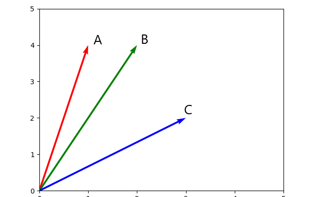
and plot them in the Cartesian coordinate system:
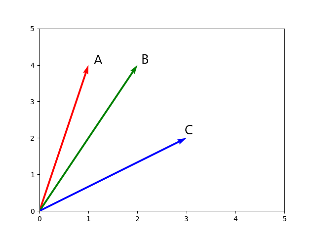
From the graph we can see that vector A is more similar to vector B than to vector C, for example.
But how were we able to tell? Well by just looking at it we see that they A and B are closer to each other than A to C. Mathematically speaking, the angle A0B is smaller than A0C.
Formula
Going back to mathematical formulation (let’s consider vector A and vector B), the cosine of two non-zero vectors can be derived from the Euclidean dot product:
$$ A \cdot B = \vert\vert A\vert\vert \times \vert\vert B \vert\vert \times \cos(\theta)$$
which solves for:
$$ Similarity(A, B) = \cos(\theta) = \frac{A \cdot B}{\vert\vert A\vert\vert \times \vert\vert B \vert\vert} $$
Solving for components
Let’s break down the above formula.
Step 1: Nominator
We will start from the nominator:
$$ A \cdot B = \sum_{i=1}^{n} A_i \times B_i = (A_1 \times B_1) + (A_2 \times B_2) + … + (A_n \times B_n) $$
where \( A_i \) and \( B_i \) are the \( i^{th} \) elements of vectors A and B.
For our case we have:
$$ A \cdot B = (1 \times 2) + (4 \times 4) = 2 + 16 = 18 $$
Perfect, we found the dot product of vectors A and B.
Step 2: Denominator
The next step is to work through the denominator:
$$ \vert\vert A\vert\vert \times \vert\vert B \vert\vert $$
What we are looking at is a product of vector lengths. In simple words: length of vector A multiplied by the length of vector B.
The length of a vector can be computed as:
$$ \vert\vert A\vert\vert = \sqrt{\sum_{i=1}^{n} A^2_i} = \sqrt{A^2_1 + A^2_2 + … + A^2_n} $$
where \( A_i \) is the \( i^{th} \) element of vector A.
For our case we have:
$$ \vert\vert A\vert\vert = \sqrt{1^2 + 4^2} = \sqrt{1 + 16} = \sqrt{17} \approx 4.12 $$
$$ \vert\vert B\vert\vert = \sqrt{2^2 + 4^2} = \sqrt{4 + 16} = \sqrt{20} \approx 4.47 $$
Step 3: Calculate similarity
At this point we have all the components for the original formula. Let’s plug them in and see what we get:
$$ Similarity(A, B) = \cos(\theta) = \frac{A \cdot B}{\vert\vert A\vert\vert \times \vert\vert B \vert\vert} = \frac {18}{\sqrt{17} \times \sqrt{20}} \approx 0.976 $$
These two vectors (vector A and vector B) have a cosine similarity of 0.976. Note that this algorithm is symmetrical meaning similarity of A and B is the same as similarity of B and A.
The above calculations are the foundation for designing some of the recommender systems.
Addition
Following the same steps, you can solve for cosine similarity between vectors A and C, which should yield 0.740
This proves what we assumed when looking at the graph: vector A is more similar to vector B than to vector C. In the example we created in this tutorial, we are working with a very simple case of 2-dimensional space and you can easily see the differences on the graphs. However, in a real case scenario, things may not be as simple. In most cases you will be working with datasets that have more than 2 features creating an n-dimensional space, where visualizing it is very difficult without using some of the dimensionality reducing techniques (PCA, tSNE).
Cosine similarity example using Python
The vector space examples are necessary for us to understand the logic and procedure for computing cosine similarity. Now, how do we use this in the real world tasks?
Let’s put the above vector data into some real life example. Assume we are working with some clothing data and we would like to find products similar to each other. We have three types of apparel: a hoodie, a sweater, and a crop-top. The product data available is as follows:
$$
\begin{matrix}
\text{Product} & \text{Width} & \text{Length} \\
Hoodie & 1 & 4 \\
Sweater & 2 & 4 \\
Crop-top & 3 & 2 \\
\end{matrix}
$$
Note that we are using exactly the same data as in the theory section. But putting it into context makes things a lot easier to visualize. From above dataset, we associate hoodie to be more similar to a sweater than to a crop top. In fact, the data shows us the same thing.
To continue following this tutorial we will need the following Python libraries: pandas and sklearn.
If you don’t have it installed, please open “Command Prompt” (on Windows) and install it using the following code:
pip install pandas
pip install sklearn
First step we will take is create the above dataset as a data frame in Python (only with columns containing numerical values that we will use):
import pandas as pd
data = {'Sleeve': [1, 2, 3],
        'Quality': [4, 4, 2]}

df = pd.DataFrame (data, columns = ['Sleeve','Quality'])
print(df)
We should get:
   Sleeve  Quality
0       1        4
1       2        4
2       3        2
Next, using the cosine_similarity() method from sklearn library we can compute the cosine similarity between each element in the above dataframe:
from sklearn.metrics.pairwise import cosine_similarity

similarity = cosine_similarity(df)
print(similarity)
The output is an array with similarities between each of the entries of the data frame:
[[1.         0.97618706 0.73994007]
 [0.97618706 1.         0.86824314]
 [0.73994007 0.86824314 1.        ]]
For a better understanding, the above array can be displayed as:
$$
\begin{matrix}
& \text{A} & \text{B} & \text{C} \\
\text{A} & 1 & 0.98 & 0.74 \\
\text{B} & 0.98 & 1 & 0.87 \\
\text{C} & 0.74 & 0.87 & 1 \\
\end{matrix}
$$
Note that the result of the calculations is identical to the manual calculation in the theory section. Of course the data here simple and only two-dimensional, hence the high results. But the same methodology can be extended to much more complicated datasets.
Conclusion
In this article we discussed cosine similarity with examples of its application to product matching in Python.
A lot of the above materials is the foundation of complex recommendation engines and predictive algorithms.
I also encourage you to check out my other posts on Machine Learning.
Feel free to leave comments below if you have any questions or have suggestions for some edits.
Continue with the the great work on the blog. I appreciate it. Could maybe use some more updates more often, but i am sure you got better or other things to do , hehe. :p